6.3 Conditional Distributions and Bayes Theorem
If f(x1, x2) is the probability function for continuous random variables (X1, X2), then
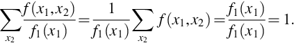
From (19) we see that
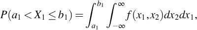
which means that
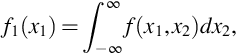
is the pdf for X1. The corresponding formulas for discrete (X1, X2) are
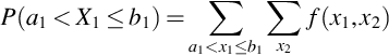
so that
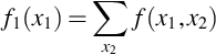
is the pmf for X1. These probability densities are distinguished by calling f(x1, x2) the joint pdf or pmf and calling f1(x1) the marginal pdf or pmf. The term joint comes from the fact that f(x1, x2) describes how X1 and X2 vary jointly. When X1 and X2 are discrete, and the sample space finite, the joint probability density can be written in a table and the sums f1(x1) are naturally written on the margins of the table.
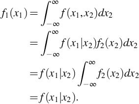
Marginal probability densities for (X1, …, Xn) are obtained from the joint density f(x1, …, xn) by integration for continuous random variables and summation for discrete random variables. The marginal probability density for continuous random variable X1 is
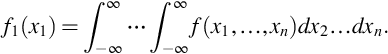
The marginal probability densities f2(x2), …, fn(xn) are also (n − 1) fold integrals.
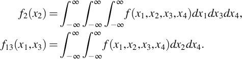
Marginal probability densities can describe two or more variables. For example, let (X1, X2, X3, X4) have joint probability density f(x1, x2, x3, x4), then the following are two of its marginal pdfs
For discrete random variables X1 and X2 the conditional probability that X2 = x2 given X1 = x1 can be defined using
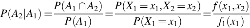
where Ai = {(x′1, x′2) : x′i = xi} and the last equality follows from the definitions of joint and marginal pmfs. It is easily checked that for any x1 such that f1(x1) > 0 the right-hand side of (20) as a function in x2 is nonnegative and sums to 1
This function is written
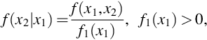
and called the conditional pmf for random variables X1 and X2. For continuous random variables X1 and X2 the joint and marginal pdfs do not provide probabilities. Nevertheless, f(x1|x2) defined in Eq. (21) will be used to defined the conditional pdf for continuous random variables X1 and X2.
Extensions to n random variables can result in joint conditional pdfs or pmfs. For example,
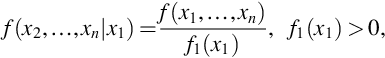
is the joint conditional pdf or pmf for X2, …, Xn given X1 = x1. The conditional pdf or pmf given Xi = xi is obtained by dividing the joint pdf or pmf by fi(xi) provided fi(xi) > 0. The conditional pdf or pmf given Xi = xi and Xj = xj is obtained by dividing the joint pdf or pmf by fij(xi, xj) provided fij(xi, xj) > 0.
Because conditional pdfs (pmfs) are pdfs (pmfs) the expectation operator can be used for these functions as well. The resulting expectation is called the conditional expectation. If X1, …, Xn are continuous random variables, the conditional expectation of u(X2, …, Xn) given X1 = x1 is

provided f1(x1) > 0 and the integral exists.
Remark 9
The marginal pdf for Xi is written fi(xi) so that when this function is evaluated at  there is no ambiguity when writing fi(a). However, the conditional distribution of Xi given Xj = xj is written f(xi|xj) and relies on the arguments to distinguish this function for different values of i and j. If Xj were observed to take the value b, f(xi|b) would be written f(xi|Xj = b). Bayes theorem describes how the conditional pdfs f(xi|xj) and f(xj|xi) are related and for that discussion it will be helpful to use the more explicit notation for two random variables X and Y
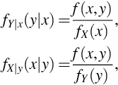
provided fX(x) > 0 and fY(y) > 0. This remark and the discussion below hold for pmfs as well as pdfs.
Bayes theorem describes how one can find fX|y(x|y0), the conditional pdf for X given Y = y0, provided we have fX(x), the marginal pdf for X, and fY|x(y|x), the conditional pdf for Y given X = x, for every value x. The proof of Bayes theorem follows directly from the definition of the conditional pdf
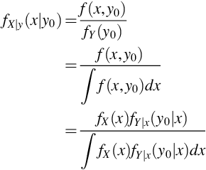
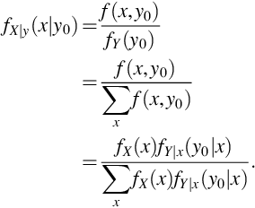
where the first equality follows from the definition of fX|y, the second from the definition of fY, and the third from the definition of fY|x. The same steps hold for discrete random variables X and Y where sums replace integration
Example 26
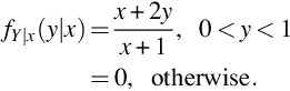
Let X and Y be continuous random variables with  and marginal and conditional pdfs given by (24) and (25).
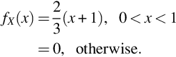
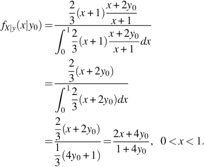
For each x between 0 and 1,
Using (22) we find
The Bayes formulas expressed in Eqs. (22) and (20) are not controversial when the random variables are functions defined on a common probability space as in Example 26. For Bayesian inference, explored in greater detail in the next chapter, a joint pdf is created from a family of pdfs by putting a distribution on the parameter space. That is, the distribution for data Y is modeled by a pdf fY(y;θ) that depends on the parameter θ which is considered an observation from a second random variable X so that
where we have used the more suggestive notation fY|θ(y|θ) for fY(y;θ) but does represent a difference of substance. The main difference from non-Bayesian inference that uses a family of probability density models {f(y;θ) : θ ∈Θ} is the marginal pdf fX(θ) on the index set Θ. This marginal pdf is called the prior and the result of Bayes formula,  , is called the posterior.
Example 27
For fixed integer n, let Y be the discrete random variables with pmf
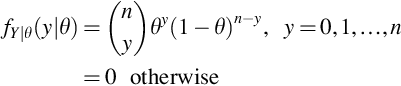
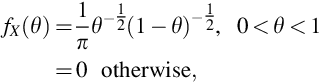
for some 0 < θ < 1. The collection of pmfs given in Eq. (26) is called the Binomial family for n trials having success parameter θ. The value θ is a realization of a continuous random variable X with marginal pdf
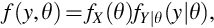
so the joint distribution is
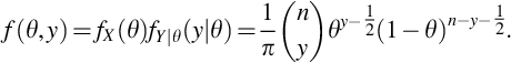
Using Bayes formula it can be shown that the posterior for each y = 0, 1, …, n is

where Γ is the gamma function.
Remark 10
The choice of prior is not necessarily obvious. One approach is to choose a prior that is, in some sense, noninformative. Jeffreys prior is one choice of noninformative prior and the distribution in Eq. (27) is Jeffreys prior for the Binomial family. Jeffreys prior and the posterior in Eq. (29) both belong to the Beta family of pdfs
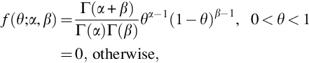
for α > 0 and β > 0. When the prior and posterior belong to the same family of pdfs, the prior and posterior are called conjugate.
7 Independent Random Variables
The  and
and  -valued random variables considered in the previous sections could be used to model a single observation taken on an individual. For example, (X1, X2, X3) could be the values obtained from measuring height, weight, and diastolic blood pressure. Statistical inference typically deals with a sample of observations. If, for example, X is bmi (body mass index) measured on an individual, then the data collected from a sample of n would be written as X1, …, Xn where Xi is the bmi for the i-th individual. If the sample of n individuals is chosen by a simple random sample then X1, …, Xn are independent random variables. We have described what it means for two events to be independent (Definition 3) and we will extend this to random variables. The observations on height, weight, and blood pressure (X1, X2, X3) would not be expected to be independent, but a sample taken on n individuals might be. To simplify notation we consider -valued random variables but this could be extended to
  -valued random variables for k > 1 . For k = 3 and a sample of n individuals the sample would be X1, …, Xn where the observation for the i-th individual is Xi = (X1i, X2i, X3i).
If random variables X1 and X2 were independent we would expect that f(x1|x2) not to be a function of x2. If f(x1|x2) is not a function of x2 then
From (30) we have
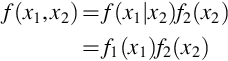
and that f(x2|x1) is not a function of x1. When this is true for all values of x1 and x2 the random variables X1 and X2 are independent. Similar calculations hold for discrete random variables X1 and X2.
Definition 11
Random variables X1 and X2 are independent if, and only if,
for all  .
.
Random variables X1 and X2 are dependent if they are not independent.
Remark 11
The equality in Definition 11 does not need to hold for all when X1 and X2 are continuous random variables. The reason is that pdfs are not uniquely defined as these functions can be changed at individual points without changing the value of the integration and it is the integration that provides probabilities. What is required is that

so that (31) holds, in some sense, almost everywhere. Measure theoretic probability makes this idea of almost everywhere precise and in advanced treatments (31) would be written
where a.e. means “almost everywhere.” This remark also applies to the equality given in Theorem 7.
To show that two random variables are independent it is often easier to use the following theorem rather than the definition which involves the marginal pdfs or pmfs.
Theorem 7
Let X1 and X2 be random variables with joint pdf or pmf f(x1, x2) with  . Then X1 and X2 are independent if, and only if,
where g(x1) > 0 for  , zero otherwise, and h(x2) > 0 for
  , zero otherwise. Note that g is only a function of x1 and h is only a function of x2.
Theorem 7 is often called the factorization theorem for independence since we need only show that the joint pdf or pmf can be factored into two functions, one that does not depend on x1 and the other does not depend on x2. Note that there is also the requirement that the sample space  is a crossproduct space. This theorem would not hold if, say,

The factorization theorem shows that the random variables X1 and X2 in Examples 22 and 23 are independent. The random variables X and Y in Examples 26 and 27 are not independent because the conditional distributions depend on the other variable.
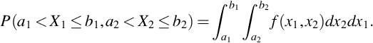
The following theorem shows that the definition of independence for random variables provides the expected relationship for events defined by these variables. That is,  when A = {(x1, x2) : a1 < x1 < b1} and B = {(x1, x2) : a2 < x2 < b2}.
Theorem 8
If X1 and X2 are independent random variables then

for all constants a1 < b1, a2 < b2.
The factorization of the joint pdf or pmf for independent random variables allows expectations to be factored for functions of the form u(X1)v(X2).

By Theorem 9 if random variables X and Y are independent then the are uncorrelated because their covariance is zero

In general, random variables being uncorrelated does not mean they are independent; independence is a stronger condition. When random variables are independent there is a restriction on the joint pdf or pmf for (almost) all values in the sample space. Uncorrelated random variables only require the expectation of one function to be zero. The definition for n independent random variables is a natural extension of Definition 11.
Definition 12
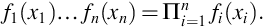
Random variables X1, …, Xn are independent if, and only if,

for all  .
.
The n-fold product in Eq. (33) will be abbreviated using the Π (product) notation
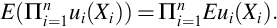
For independent random variables X1, …, Xn Theorem 8 becomes

and Theorem 9 becomes
8 Central Limit Theorem
The central limit theorem can be described informally as a justification for treating the distribution of sums and averages of random variables as coming from a normal distribution. It should be noted that the central limit theorem is a theoretical result for what holds when the number of random variables n goes to infinity. While this theorem is not about any finite number n of random variables, in practice, the normal approximation to the sample mean (and related quantities, such as slopes in linear regression) is often very good even for modest values of n. For data that are not highly skewed and for which there are no extreme outliers, samples of size 30 or larger are considered large enough to use the normal approximation. There are many versions of the central limit theorem and the one we consider here is for the sample mean  , where X1, …, Xn are not only independent but also identically distributed which means the marginal pdfs or pmfs are all the same
When the random variables X1, …, Xn are independent and have identical probability distributions they are called a random sample. We assume the first two moments of f(x) exists and write
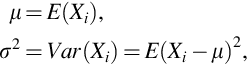
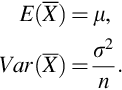
where i and be any value from 1, 2, …, n. From the properties of the expectation operator for independent random variables it is easily shown
To discuss the central limit theorem we need to defined what is meant by a limiting distribution whose distribution depends on n.
Definition 13
Consider a sequence of random variables Yn whose probability distribution function Fn(y) depends on integer n > 0. If F(y) is a probability distribution function and if
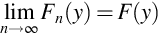
for every continuity point of F(y), then Yn is said to have a limiting distribution with probability distribution function F(y).
Theorem 10
Let X1, …, Xn be a random sample from a distribution having mean μ and standard deviation σ > 0.
Then the standardized version of  , namely,
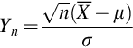
has a limiting distribution that is normal with mean 0 and standard deviation 1.
Note that for each n, E(Yn) = 0 and V ar(Yn) = 1. What changes with n is the shape, and in the limit the shape of the probability distribution function for Yn is that of the normal distribution.
The assumption that each Xi have the same distribution can be dropped but other assumptions must be made. An important application where the distributions are not identical is for regression. For normal linear regression, Y1,…, Yn are independent but fi(yi) = f(yi, μi) where f(y, μi) is the normal distribution with mean μi and standard deviation σ that is the same for all i. When μi is a linear function in the covariates Xi = (Xi1, …, Xik) this is normal linear regression and has important properties for statistical inference. In particular, normal linear regression has sufficient statistics that are not a function of the number of observations n. Sufficiency will be discussed in the next chapter.
Generalized linear models are an extension of normal linear regression to probability distributions from an exponential family. In a generalized linear model the pdf or pmf f(y, μi) is a member of an exponential family having mean parameter μi and a transformation of μi is linear in Xi. This transformation is called the link function and for each exponential family there is an important function called the canonical link. When the canonical link is used, generalized linear models will have sufficient statistics that do not depend on n.