Machine Learning
Gangadhar Shobha1; Shanta Rangaswamy1 R. V. College of Engineering, Bengaluru, India
1 Corresponding authors: email address: shobhag@rvce.edu.in, shantharangaswamy@rvce.edu.in
Abstract
The objective of this chapter is to provide the reader with an overview of machine learning concepts and different types of learning techniques which include supervised, unsupervised, semi-supervised, and reinforcement learning. Learning algorithms discussed in this chapter help the reader to easily move from the equations of the book to a computer program. Various metrics like accuracy, precision, confusion matrix, recall, RMSE, and quantile of errors used to evaluate machine learning algorithms are outlined in this chapter. At the end of this chapter we present various applications of machine learning techniques followed by future trends and challenges.
Keywords
Learning model; Machine learning; Algorithms; Regression; Metrics; Decision tree
1 Introduction to Machine Learning
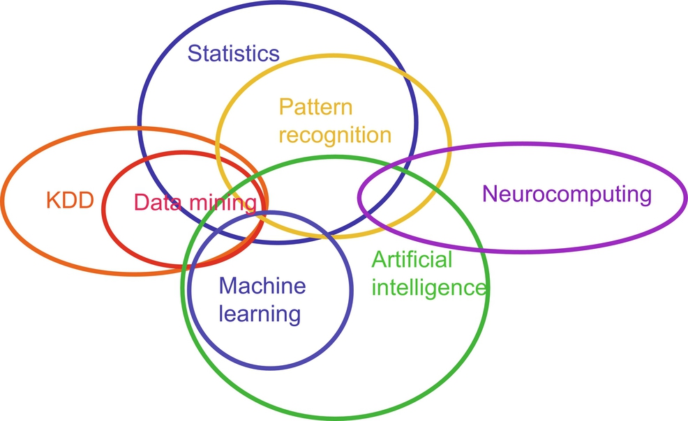
Machine learning is a subfield of Artificial Intelligence (AI) and has evolved from pattern recognition, used to explore the structure of the data and fit into the models which can be understood and utilized by users. It answers the question as to how to construct a computer program using historical data, to solve a given problem and automatically improve the efficiency of the program, with experience. In the recent years, various machine learning applications have been developed, like model to classify new astronomical structures, detecting fraudulent banking transactions, information-filtering systems that learn user reading preferences, neurobiological studies, autonomous vehicles that learn to drive on highways. Also at the same time, there has been an important progress in the concepts and the algorithms that form the foundation of machine learning. Fig. 1 is an indicative representation of degree of similarities and dissimilarities among the various fields of computer science.
In conventional or traditional way of computing, algorithms are the set of explicitly programmed instructions used by computers to calculate or solve a problem. When compared to traditional way of computing, machine learning algorithms facilitate computers to build model from sample data available, and to automate decision making process, based on data inputs and experience. These techniques identify patterns in data and provide various tools for data mining.
Today, every technology user is at an advantage from machine learning. The technology of facial recognition allows social media to tag its users. Recommendation engines suggest which movies or television shows to watch next based on user preferences. Optical Character Recognition (OCR) technology converts images of text into editable type. Self-driving cars depend on machine learning to navigate its way, may soon be available to consumers. Thus, machine learning is a continuously evolving and developing field, wherein some known and unknown challenges need to be analyzed.
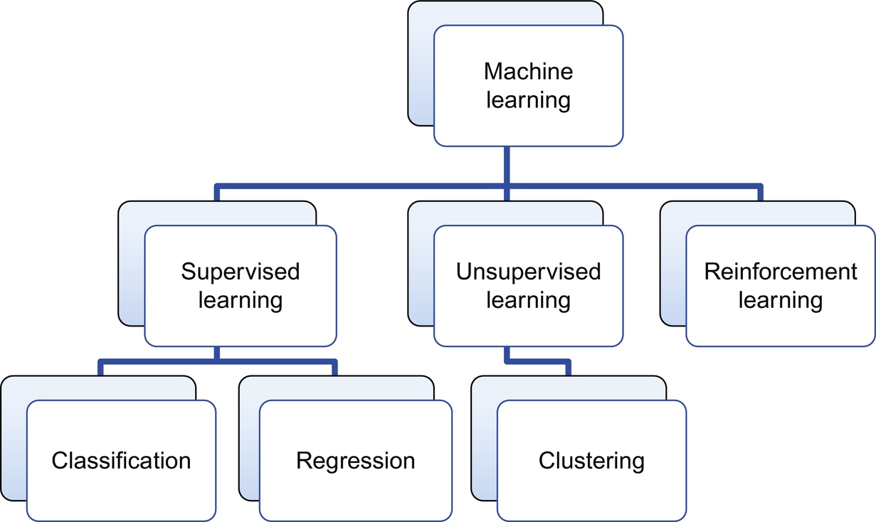
Machine learning is broadly classified as supervised, unsupervised, semi-supervised, and reinforcement learning. A supervised learning model has two major tasks to be performed, classification and regression. Classification is about predicting a nominal class label, whereas regression is about predicting the numeric value for the class label. Mathematically, building a regression model is all about identifying the relationship between the class label and the input predictors. Predictors are also called attributes. In statistical terms, the predictors are called independent variables, while the class label is called dependent variable. A regression model is a representation of this relationship between dependent and independent variables. Once this is learnt during the training phase, any new data is plugged into the relationship curve to find the prediction. This reduces the machine learning problem to solving a mathematical equation. The broad classification of machine learning is depicted in Fig. 2.
1.1 Supervised Learning
Supervised learning is a learning model built to make prediction, given an unforeseen input instance. A supervised learning algorithm takes a known set of input dataset and its known responses to the data (output) to learn the regression/classification model. A learning algorithm then trains a model to generate a prediction for the response to new data or the test dataset. Supervised learning uses classification algorithms and regression techniques to develop predictive models. The algorithms include linear regression, logistic regression, and neural networks as well, apart from decision tree, Support Vector Machine (SVM), random forest, naive Bayes, and k-nearest neighbor.
Classification task predicts discrete responses. It is recommended if the data can be categorized, tagged, or separated into specific groups or classes. Classification models classify input data into categories. Popular or major applications of classification include bank credit scoring, medical imaging, and speech recognition. Also, handwriting recognition uses classification to recognize letters and numbers, to check whether an email is genuine or spam, or even to detect whether a tumor is benign or cancerous.
Regression techniques predict continuous responses. A linear regression attempts to model the relationship between two variables by fitting linear equation to observed data. For example, say, a data is collected about how happy people are after getting so many hours of sleep. In this dataset, sleep and happy people are the variables. By regression analysis, one can relate them and start making predictions.
In Natural Language Processing, the input can contain an annotated text provided by humans. Annotated text is a metadata that is given along with the dataset to the machine. The annotations can be Part-of-Speech tagging (PoS tags), phrase, and dependency structures. For example, to determine whether the text “clean dishes” is a noun phrase or a verb phrase, the algorithm needs to be trained using annotated sentences like “Clean dishes are in the cupboard” or “Clean dishes before going to work.” In the first case, the annotation says that it is a noun phrase and verb phrase in the second case.
1.2 Unsupervised Learning
In supervised learning, the goal is to learn mapping from the input to an output whose correct values are provided by a supervisor. But, in unsupervised learning, the goal is to find the regularities in the input such that certain patterns occur more often than others and to learn to see what generally happens and what does not. Examples on speech recognition, document clustering, and image compression go well with unsupervised learning. In document clustering, the aim is to group documents into various reports of politics, entertainment, sports, culture, heritage, art, and so on. Usually any document is represented as a “bag of words,” that is, predefined lexicon of N words. Each document is an N-dimensional binary vector whose element “I” is 1. If the word “I” appears in the document, its suffixes “-s” and “-ing” are removed to avoid duplicates and stop words such as “of,” “and,” “the,” “a” are also removed. Remaining terms in the document are then grouped, depending on the number of shared words.
1.3 Semi-supervised Learning
This learning technique is the combination of supervised and unsupervised learning and is used when less number of labeled data is identified for a particular application. It generates a function mapping from inputs of both labeled data and unlabeled data. The goal of semi-supervised learning is to classify some of the unlabeled data using the labeled information set. In a semi-supervised learning scenarios, the size of the unlabeled dataset should be substantially larger than the labeled data. Otherwise, the problem can be simply addressed by using supervised algorithms. Some real world examples like, protein sequence classification, web content classification and speech analysis where labeling audio files is a very intensive task and requires lot of human intervention.
1.4 Reinforcement Learning
Reinforcement learning involves interacting with the surrounding environment. Reinforcement learning addresses the issue of how an autonomous agent that senses and acts in its environment can learn to choose optimal actions to achieve its goals. An agent's behavior is rewarded based on the actions it takes in the environment. It considers the consequences of its actions and takes optimal steps further. A computer playing chess with the human, learning to recognize spoken words, and learning to classify new astronomical structures are few examples of reinforcement learning.
2 Terminologies
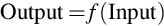
The statistical perspective of machine learning frames data in the context of a hypothetical function (f) that the machine learning algorithm aims to learn. Given an input variable (input) the function answers the question as to what is the predicted output variable (output).
In terms of database, row of a data describes an entity or an observation about an entity. The column for a row is referred as attribute of an observation and rows are the instances. Variables are the properties or the kind of characteristics of a certain event or object in a dataset. It could be dependent or independent variables. Independent variables are the one that can be manipulated or changed by researchers or data analyst and then its effects are measured and compared with. Independent variables are also known as Predictor(s). Independent variables are called so because they predict or forecast the values of the dependent variable in the model. The dependent variables refer to the type of variable that measures the effect of the independent variable(s) on the test units. Dependent variable is also known as predicted variable because they are the values that are predicted or assumed by the predictor or independent variables.
Consider a scenario where a student's score in an examination is a dependent variable, as it may change depending on several factors, like how much he has studied a particular subject, how much he slept in a night before the exam, or how hungry he was when he took the exam. Generally, when an analyst is looking for a relationship between two things, he is trying to figure out what makes the dependent variable change the way it does.
3 Regularization and Bias–Variance Trade-Off
The main intend of machine learning is to build a model that performs well on both the training set and the test set. Once a machine learning model is built, there are number of ways to fine-tune the complexity of the model. Regularization is about fine-tuning or selecting the preferred level of model complexity so that the model performs better at prediction (generalization). Generalization is a concept in machine learning which tells how well the model performs on new data or on the data that is previously unseen. A model with strong generalization ability can form the whole sample space very well.
Training set: Training set or dataset is the data used for training the model.
Validation set: The available dataset is randomly divided into training set and validation set. The model is fit on the training set, and the fitted model is used to predict the responses for the observations in the validation set. The resulting validation set error rate is assessed using Mean Squared Error (MSE) to provide an estimate of the test error rate.
Testing set: Test data or test set is the data used for testing the model already built. This data may or may not be similar to training dataset values. The error on the test data indicates how well the classifier performs on new data. This is generalization, and the test error is known as generalization error.
Overfitting is a scenario when the classifier has low training error and high testing error. In case of overfitting, a classifier or a model tries to capture every sample point instead of genuine sample at the point. Suppose a classifier model is built using decision tree approach. The size (length and width) of the tree built would mainly depend on the number of features and the number of instances in the dataset. Too small or too large tree may not be favorable in terms of accuracy and the speed at which it reaches a class label. Also the tree built may have a high accuracy on the training data, but very less accuracy on the test data. This scenario is known as Overfitting. Two optimal approaches or solution to avoid overfitting could be: (i) prepruning, that is, halt the tree construction early. Do not split a node if this would result in the goodness measure falling below a threshold, as it is difficult to choose an appropriate threshold, and (ii) postpruning, that is, removing branches from a fully grown tree, and get a sequence of progressively pruned trees.
Variance: When a model performs really well on training dataset and poorly on cross-validation data, then the model is said to have variance. This means the model is overfitting (making a complicated model so that it fits the training data very well). Potential solution to overcome variance could be: Get more training data (if possible), try smaller features (by reducing the order of polynomial or number of layers in neural network), and increase regularization parameter (that is, penalize the features). An example for high-variance algorithm is k-nearest neighbors algorithm, while Linear Discriminant Analysis (LDA) is an example of a low-variance algorithm.
Underfitting: Underfitting of the curve occurs when a model is too simple and informed by very less features or regularized too much, which makes the model rigid toward learning from the dataset. Simple learners have a tendency to have less variance in their predictions, but more bias toward wrong outcomes. Underfitting scenario happens, when learner has not found a solution that fits the observed data to an acceptable level, for example, if the learning time is too large, and the learning stage is prematurely terminated, or if the learner did not use a sufficient number of iterations, or if the learner tries to fit a straight line onto training set whose examples exhibit a quadratic nature. A model that underfits the training data will miss important aspects of the data, and this will negatively impact its performance in making accurate predictions on new data it has not seen during training.
Bias: A learning model is said to have bias when it performs poorly on the training data as well as on the cross-validation data. Potential solution to overcome bias could be: Make a complicated (bigger) model (by having neural network with more layers or polynomial features), train the dataset longer, or decrease regularization parameter. Using more examples will not have much influence on the model, as the model is already inadequate and underfits (bias) the training data. Decision tree is an example of a low-bias algorithm, and linear regression is an example for high-bias algorithm.
4 Evaluating Machine Learning Algorithms
Classification is the process of finding a model that describes and distinguishes data class labels. A model is derived based on the analysis of a set of training data (objects for which the class labels are known). It is used to predict the class label of objects for which the class label is unknown. A well-known classifier, decision tree, is a flow chart like tree structure, where each node denotes a test on an attribute value, each branch represents an outcome of the test, and tree leaves represent classes or class distributions. In binary classification, there are two possible output classes. One common example of classification is spam detection in an email inbox, where an input set is an email received along with its metadata (sender's name and sent time), and the output label is either “spam” or “not spam.” One may also use generic names for the two classes as “positive” and “negative” or class “1” and class “0.” There are different ways of evaluating the performance of classification. Accuracy, confusion matrix, precision, and recall are the widely used evaluation metrics.
4.1 Accuracy
Accuracy is the amount of correctly classified instances of the total instances. It is defined as the ratio of number of correct predictions to the total number of predictions. However, if the test data is not balanced (that is, when most of the instances or records belong to one of the classes), or one is more interested in the performance on either one of the classes (biased), the accuracy metric will not be able to capture the effectiveness of a classifier. For example, in an employee income level classification scenario, a data analyst is testing on some data where 99% of the instances represent employees who earn less than or equal to 50K per annum. It is possible to achieve an accuracy of 0.99 by predicting the class “≤ 50K” for all instances. The classifier in this scenario seems to be doing well, but in reality fails to classify any of the high-income individuals correctly (top 1%).
4.2 Confusion Matrix
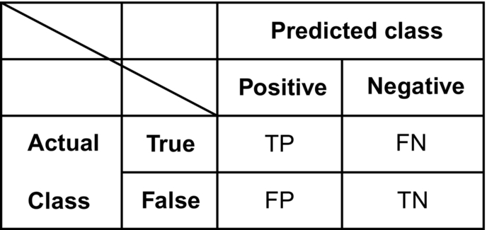
It is a table that records the number of instances in a dataset that fall in a particular category. The class label in a binary training set can take two possible values, which are called as positive class and a negative class. As seen in Fig. 3, the number of positive and negative instances that a classifier predicts correctly is called True Positives (TP) and True Negatives (TN), respectively. The misclassified instances are known as False Positives (FP) and False Negatives (FN). A learning model involuntarily decides which two classes in the dataset is the positive class. If the class labels of a dataset are strings, first the label is sorted alphabetically and at the first level, it is chosen as a negative class, while in the second level it is chosen as positive class. If the class labels are boolean or integer in nature, then “1” or “true” labeled instances are assigned as positive class.
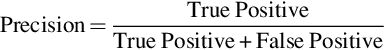
4.3 Precision and Recall
Precision is the fraction of relevant instances among the retrieved instances.
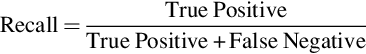
Recall (opposite of precision) is not so much about answering questions correctly but more about answering all questions that have answer “true” with the answer “true.” Therefore, if the models always answer “true,” it is 100% recall.
It is important to note that measures precision and recall do not provide any information on the number of true negatives. This means it can be the case that a person has lousy precision and recall score (e.g., 50%) and still answered 99.99% of all questions correctly.
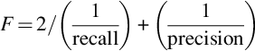
4.4 F Measure
In statistical analysis of binary classification, the F score (or F measure) is a metric of a test's accuracy. It takes into consideration the precision and the recall of the test to compute its score. F measure is the harmonic average of precision and recall. F measure reaches its best value at 1 (perfect precision and recall) and worst at 0.
4.5 Regression Metrics
In any regression task of supervised learning, the model learns to predict numeric scores. For example, when an individual tries to predict the price of the stock in the coming days, given the past history of the company and the market, it can be treated as a regression task. RMSE and quantiles error are the major evaluating metric for regression. Quantile plots are used for univariate data distribution.
RMSE: RMSE is defined as the square root of the average squared distance between the actual score and the predicted score
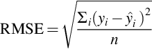
where yi is the true score for the ith data point, ŷi is the predicted value, and n is the number of data points.
RMSE measures the standard deviation of the predictions from the ground truth. The RMSE is one way to measure the performance of a classifier. Error rate (or number of misclassification) is another one. It is not recommended to use RMSE as the sole means to understand how well classifier is performing. RMSE usually gives us how distant our model is from giving the right answer. So, in a binary classifier, the square root of the mean of the sum of all the instances (each instance will be 1 or − 1) where a binary classifier has gone wrong will be a number between in the scale 0 to 1, indicating how good (closer to 1) or how bad (closer to 0) the classifier is performing. It is mostly used for regression problems. For classification, classification accuracy is a more appropriate measure.
Quantiles of errors: RMSE comes with a disadvantage, as it takes mean of all the data points. Assuming the dataset consists of an outlier, it will have a major impact on the average value. The effect of large outliers during evaluation can be reduced by using robust metric called quantiles of errors. It considers Median Absolute Percentage Error

4.6 k-Fold Cross-validation
It is understood that more the training data, lesser will be the error rate; hence it is not advised to reduce the training set data. Also, one may lose important patterns by increased bias in a model. So, we would like to have a method, which can increase the data used for validation without reducing the training set data. This can be achieved using k-fold cross-validation, where the data is divided into k-folds. In this approach, one has to carry out holdout method repeatedly, where each time one of the k-folds is used as the validation data and the remaining k − 1 folds is used as the training set. The error approximation is obtained by calculating the average over K trials. The same is depicted in Fig. 4
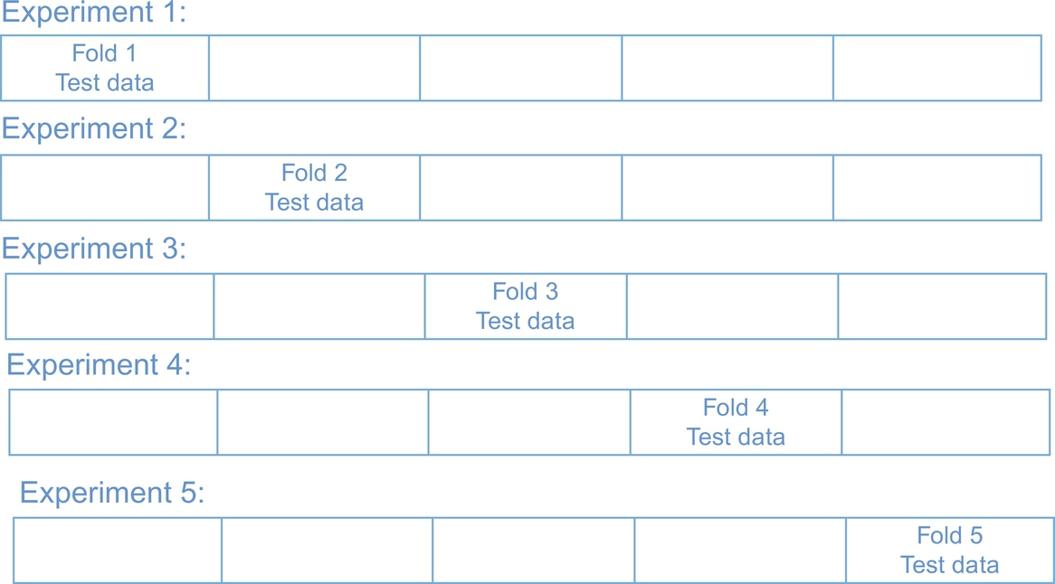
For example, if 1000 product reviews are collected, these are split into k = 10-folds. Therefore, each fold = 100 reviews.
- First fold = review no. 1 to review no. 100, second fold = review no. 101 to review no. 200,
- Third fold = review no. 201 to review no. 300, and so on.
Therefore, in the first experiment, first fold is considered as test data and all other ninefolds are used for training, which means first hundred reviews are fed as input to system, before which remaining 900 reviews are stored in system database, with sentimental numbers (1, − 1) assigned to them. Such experiments are conducted 10 times by selecting a different fold for test data in every experiment. Average of error estimated in each experiment is calculated.
4.7 Stratified k-Fold Cross-validation
There are some instances where the dataset may be skewed toward a particular value. For example, in a dataset of a rare disease, there might be large number of negative predictions than positive ones. In such scenarios, k-fold validation does not perform well, and a variation of k-fold validation is used, where there is equal representation of each type of class label, and we also make sure each fold has the same percent of representation as well. This type of validation is called as stratified k-fold cross-validation.
4.8 Advantage and Disadvantage of Cross-validation
The major advantage of using cross-validation is that it is conceptually simple and easy to implement. However, it also suffers from certain disadvantages. The first disadvantage is that when we use this method, the validation set error rate can be highly variable. Second, only subsets of the observations (those in the training set) are used to fit the model. As machine learning methods tend to perform poor when trained on fewer observations, validation set error rate may tend to overestimate the test error for the model fit on the entire dataset.
4.9 Bootstrapping and Bagging
Bootstrapping is a resampling technique, where a data analyst repeatedly draws different samples from the same dataset. Thus, using this validation scheme, it is possible to get a better idea of the representation of class labels present in the dataset. Here, we draw samples from a dataset such that it increases the size of test data and resample it (with replacement) from the training data that produces a fairly larger amount of “phantom samples” or bootstrap samples.
Bagging aggregates the fitted values in various ways. Ideally, many sets of fitted values, each with low bias but high variance, may be averaged in such a way that they can effectively reduce a bit of the bias–variance trade-off.
5 Regression Algorithms
Machine learning algorithms can also be divided as parametric learning model and nonparametric learning model. Algorithms that have strong assumptions in the learning process and that simplify the function to the known form are known as parametric machine learning algorithms. Linear regression and logistic regression are the examples of parametric machine learning algorithms. Regression algorithms deal with modeling the relationship between variables that are refined iteratively using a measure of error in the predictions made by the model. Linear regression is an approach to model the relationship between a scalar-dependent variable y and one or more explanatory variables (or independent variables) denoted x. Linear and logistic regressions are the major algorithms in predictive modeling.
Linear regression is a popular way of analyzing data described in a model which is linear in nature. It is a process of finding the optimal fitting straight line through the given data points. However, a mathematical representation relates the response to the predictor variables. Linear regression is an attempt to model the relationship between two variables by fitting a linear equation to observed data, where one variable is considered to be an explanatory variable and the other as a dependent variable. For example, statistician may want to relate the weights of individuals to their heights using a linear regression model.
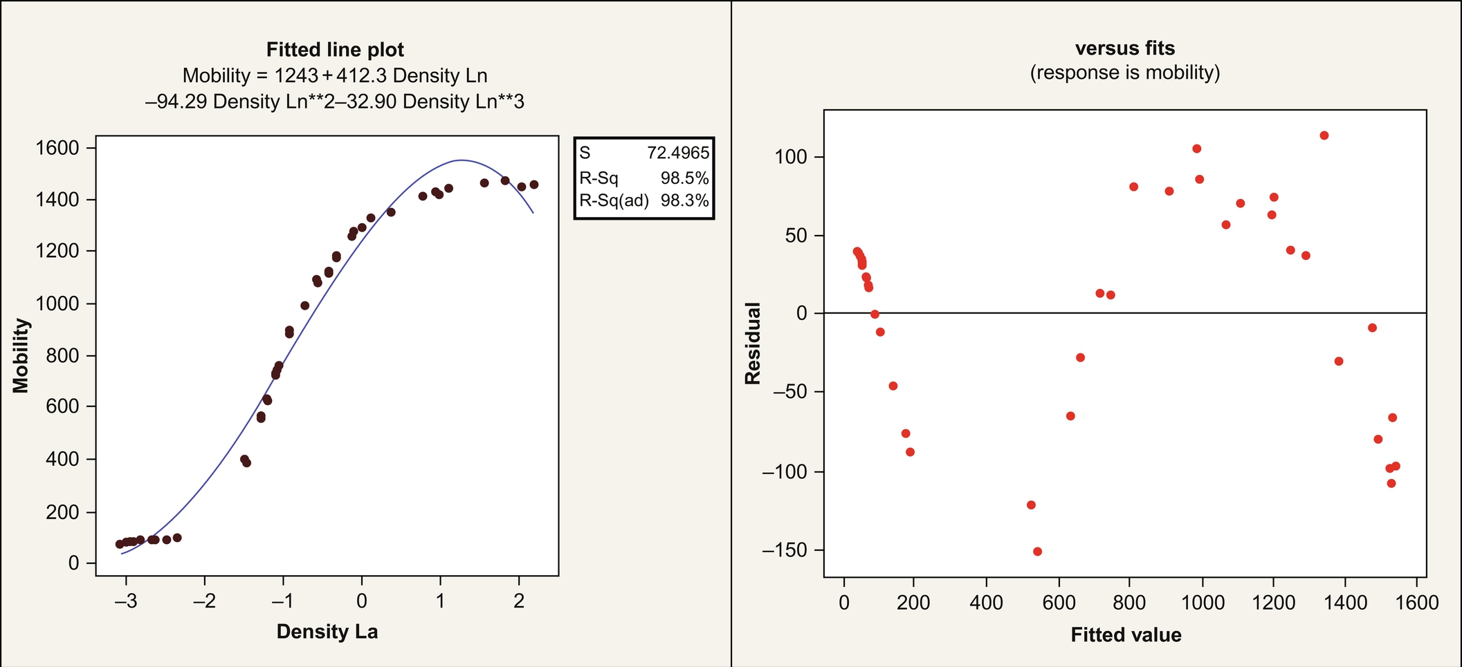
A simple linear regression relates two variables (x and y) with a straight line equation, while a nonlinear regression generates a line, as if every value of y is a random variable. The objective of this model is to make sum of the squares value as small as possible. Linear regression is easier to use and interpret. However, if good fit with linear regression is not possible, then nonlinear regression is used. Logarithmic functions, exponential functions, and trigonometric functions are among the other fitting methods in a nonlinear regression. The graphical representation of linear regression is seen in Fig. 5.
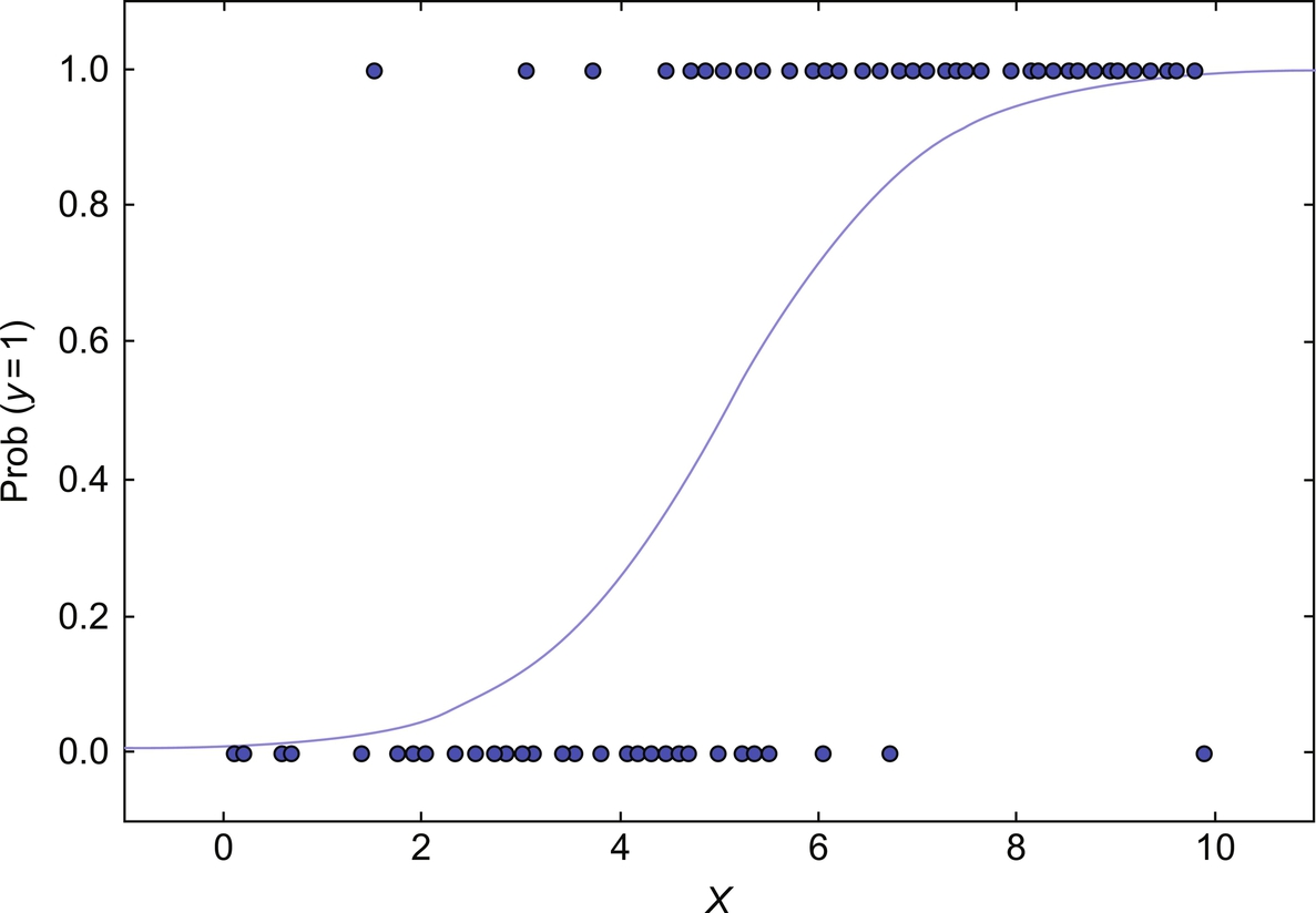
Logistic regression: Logistic regression is used to estimate the probability of event being “success” and event being “failure.” One should go for logistic regression when the dependent variable is binary in nature.
The value of y is from 0 to 1 and can be represented as:
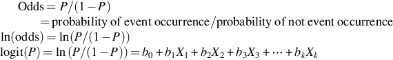
P estimates the probability of existence parameter of interest. Logit function chooses a link function that is very appropriate for this kind of distribution. Fig. 6 shows an example of logistic regression between two variables x and y, which lies between 0 and 1.
Other types of regressions available are polynomial regression, stepwise regression, ridge regression, lasso regression, and elastic net regression.
6 Classification Algorithms
As discussed earlier, classification is a supervised mode of building a model. Algorithms that do not make any strong assumptions or hypotheses about the form of the mapping function are called as nonparametric machine learning algorithms. Nonparametric methods are usually more flexible and achieve better accuracy but require huge data and training time. SVMs, Neural Networks, and Decision trees are the examples of nonparametric algorithms.
6.1 Decision Tree Algorithm
The purpose of building a decision tree is to predict the target variable based on the input variable by learning decision rules. Decision trees are commonly used for classifying the data and also in regression. Classification tree models yield discrete set of values for target variables, while regression tree models take continuous set of values for target variables.
To build a model of the classifying attribute based upon the other attributes the decision tree takes an object as input which is described by a set of properties. The decision in each stage of the tree depends on the previous branching operations. The tree building starts with the root node, then performs the test that follows the edge, and repeats the test till it reaches end (leaf) node. Once it reaches the leaf node, the tree predicts the outcome associated with it, that is, class label. ID3 and its successor C4.5 are the benchmark algorithms for decision trees.
Sample example:
Consider a car dataset for classification using decision tree classifier. Here the class labels are positive and negative, as shown in Fig. 7.
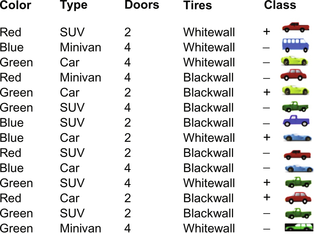
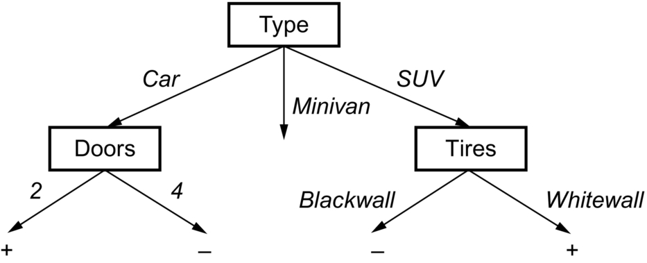
Drawing a decision tree from the available dataset involves splitting attribute of each node. Each branch will have a possible value of the corresponding attribute. Splitting attribute is the most informative attribute among all the attributes. To select the most informative attribute, an algorithm uses a factor called Entropy. Goodness of a split is determined by information gain. Attribute with the maximum information gain is considered to split. Dataset is split for all the attributes values. Fig. 8 indicates the sample decision tree built from the dataset.
6.1.1 A Good Selection of Attribute
A good attribute is the one which splits the data such that each successor node is as pure as possible, that is, the distribution of instances of the dataset in each node must contain instances of a single class. Information gain, Gini index, and gain ratio are the popular methods by which the node attribute of a decision tree is decided.
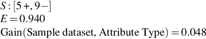
6.1.2 Entropy
The partitioning of dataset into subset must contain instances whose values are homogenous. Iterative Dichotomiser 3 (ID3) and C4.5 (successor of ID3) are specific decision tree algorithms that use entropy as an attribute selection method. Entropy is used to measure the homogeneity of the samples that characterize the purity of a dataset. It is also defined as the amount of information contained in an attribute. Fig. 9 represents the form of the entropy function, as probability varies between 0 and 1.
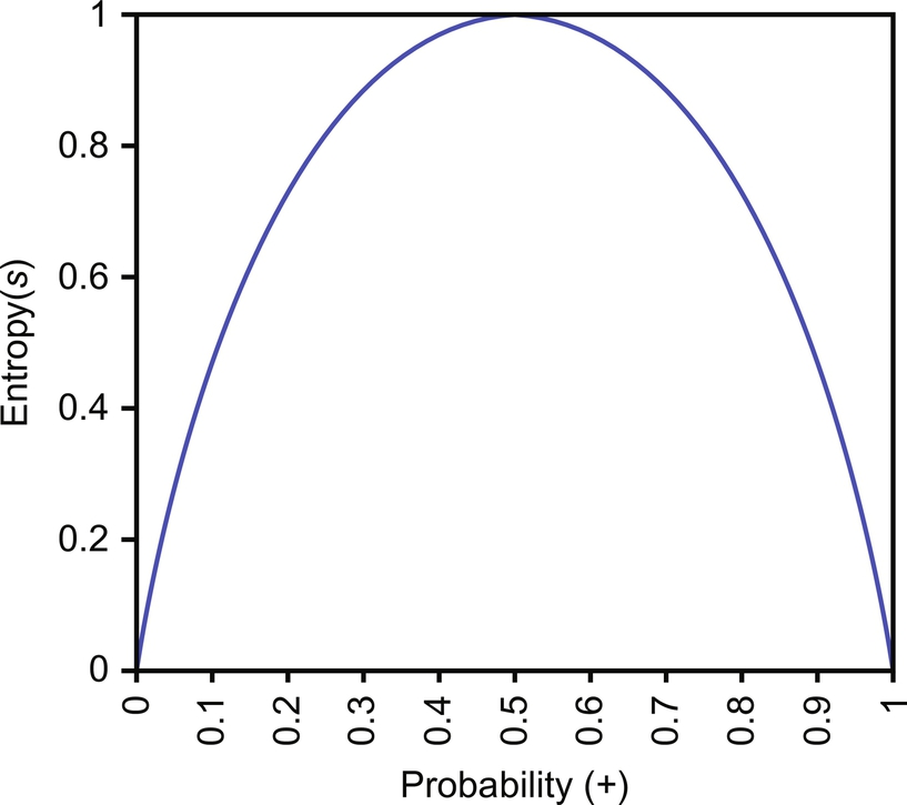

Consider a dataset S consisting of training examples of two classes, namely, positive and negative.
P+ denotes the proportion of positive examples in S
P− denotes the proportion of negative examples in S
Impurity of S is measured by entropy.

6.1.3 Information Gain
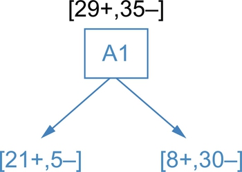
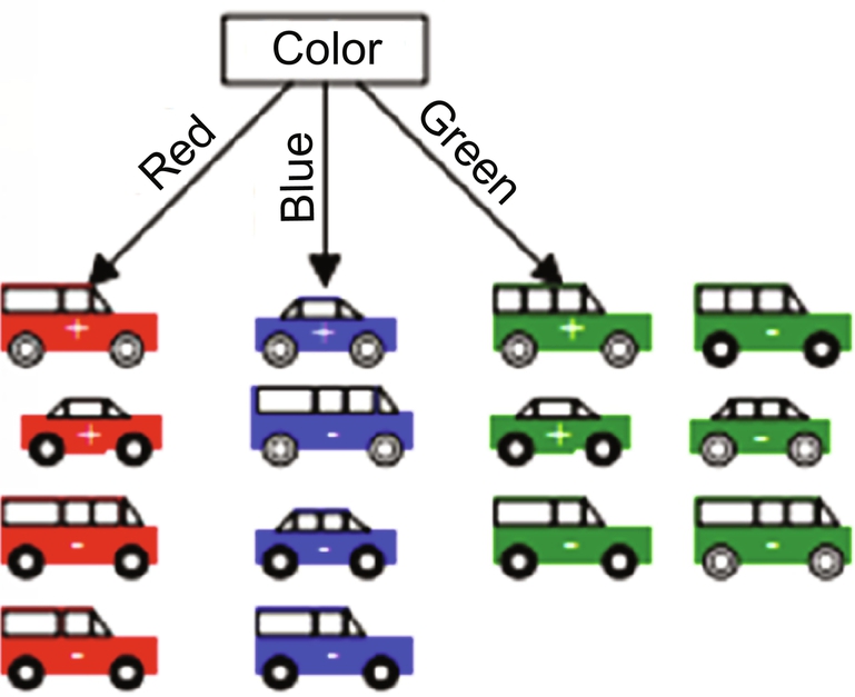
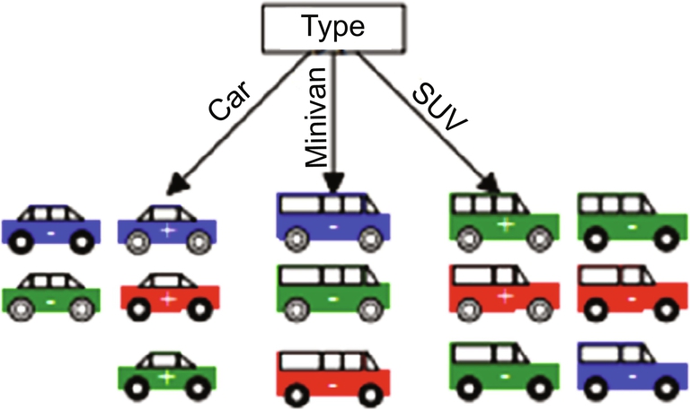
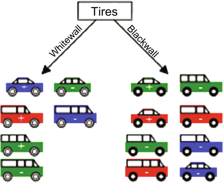
Information gain is based on entropy. Gain (Sample dataset, Attribute) is the expected reduction in an entropy because of sorting on an attribute. Figs. 10–14 shows the flow or sequence in which a decision tree is formed for a sample dataset.

Example:
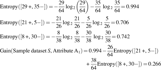
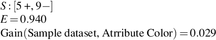
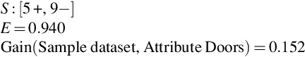
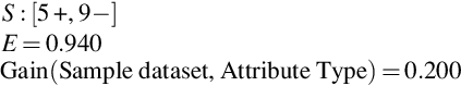
Best attribute among Color, Type, Doors, and Tires is the attribute Type with Gain equal to 0.200
6.1.4 Gini Index
The well-known decision tree algorithm Classification And Regression Trees (CART) uses Gini index as an impurity (or purity) measure in building the decision tree. It is an alternative measure for information gain.
Impurity measure which is used instead of entropy is given by:

where Pi is the probability that a tuple in D belongs to class Ci and is estimated by | Ci,D |/|D |. The sum is computed over m classes.
6.1.5 Pruning of a Tree
The greed to fit data using decision tree can sometimes result in overfitting of data. To avoid this, a strong stopping criterion or pruning is to be used. Pruning is exactly opposite of splitting. Pruning can be carried out by top-down approach or bottom-up approach.
6.1.6 Representing a Decision Tree
An attribute is tested at each internal node. The attribute value corresponds to the branch of the classification label and is assigned by the leaf node. An example is classified by sorting it through the tree from root to leaf.
Example:

Tree to rules
A set of rules can be constructed from its equivalent tree. Each rule is formed from each leaf node of the tree. Each rule is pruned independently from other rules. Finally, a desired sequence for use is obtained by sorting the final rule.
- Rule 1: IF (Type = Car) ⋀ (Doors = 4) THEN class +
- Rule 2: IF (Type = SUV) ⋀ (Tires = Black wall) THEN class −
- Rule 3: IF (Type = Minivan) THEN class −
6.1.7 Advantages of Decision Tree
- 1. Decision trees are simple to understand, interpret, and visualize.
- 2. It implicitly performs variable feature selection.
- 3. Numerical and categorical data can be handled efficiently.
- 4. Data preparation can be done without any effort from users.
- 5. Performance of the tree is not adversely affected by the nonlinear relationship of the parameters.
- 6. It is easy to add expert preferences, opinion, and hard data.
- 7. Decision techniques can be easy incorporated with decision tree.
- 8. Decision trees are very flexible so that they can easily adopt to new scenarios.
6.1.8 Disadvantages of Decision Tree
- 1. More information gain is obtained with more levels when categorical variables with multiple levels are used.
- 2. Complex calculations are needed and it is the only problem when tree is created by hand.
- 3. Overfitting is the major problem in decision tree as highly complex tree is created where the data is not generalized well.
- 4. If the data changes slightly, a small variation results in different tree and this makes decision tree unsuitable as it is unstable. It is known as variance. Variance can be reduced by the methods like boosting, bagging.
- 5. It is not guaranteed that the greedy algorithm will not always return globally optimal decision tree. To overcome this, the samples can be randomly sampled to train multiple trees.
- 6. Biased tree can be constructed when some classes dominate. To mitigate this, it is better to balance the training dataset to fit the decision tree model.
6.2 Naive Bayesian Classification
Naive Bayes is a simple and powerful algorithm for predictive modeling. The model comprises two types of probabilities that can be calculated directly from the training data: (i) the probability of each class and (ii) the conditional probability for each class given each x value. Once calculated, the probability model can be used to make predictions for new data using Bayes theorem. When the data is real valued, it is common to assume a Gaussian distribution (bell curve) so that one can easily estimate these probabilities. Naive Bayes is called naive because it assumes that each input variable is independent. This is a strong assumption and unrealistic for real data; however, the technique is very effective on a large range of complex problems. The thought behind naive Bayes classification is to try to classify the data by maximizing P(O | Ci)P(Ci) using Bayes theorem of posterior probability (where O is the Object or tuple in a dataset and “i” is an index of the class). The steps of implementing Bayes classifier are as follows:
- Step 1: Let D be a training set of tuples or Objects O and their associated class labels. Each tuple is represented by an n-dimensional attribute vector. O = (o1, o2, …, on) depicts n measurements made on the tuple from attributes A1, A2, A3, …, An, respectively.
- Step 2: Assuming there are m classes, C1, C2, …, Cn, given a tuple O, the classifier will predict that O belongs to the class having the highest posterior probability conditioned on O. That means the naive Bayesian classifier predicts that tuple O belongs to the class Ci if and only if P(Ci | O) > P(Cj | O) for 1 ≤ j ≤ n, j ≠ i.
- That is, we maximize P(Ci | O). The class Ci for which P(Ci | O) is maximized is called maximum posteriori hypothesis. Applying Bayes theorem,
- Step 3: As P(O) is constant for all classes, only P(O | Ci)P(Ci) needs to be maximized. If the class prior probabilities are not known, then it is assumed that the classes are equally likely, that is, P(C1) = P(C2) = … = P(Cn) and we would therefore maximize P(O | Ci). Otherwise, one has to maximize P(O | Ci)P(Ci). Also the class prior probabilities may be estimated by P(Ci) = | CiD |/|D |, where | CiD | is the number of training tuples of class Ci in D.
- Step 4: Now, given the dataset with many attributes, it would be computationally expensive to compute P(O | Ci). To reduce the computation of evaluating P(O | Ci), the naive assumption of class independence is made. This presumes that the attribute values are conditionally independent of one another, given the class label of the object (that is, there are no dependent relationships among the attributes). Thus,

- Step 5: To predict the class label of O, P(O | Ci)P(Ci) is evaluated for each class Ci. The classifier predicts that the class label of tuple O is Ci if and only if

One may estimate the probabilities of P(oi | Ci), P(o2 | C2), ..., P(on | Ci) from the training tuples.
For example, a fruit can be considered to be an apple, if it is red, round, and approximately 10 cm in diameter. A naive Bayes classifier considers each of these features independently to the probability that the given fruit is an apple, irrespective of any possible correlations between the color, shape, and diameter.
6.3 Support Vector Machine
SVM is one of the best known algorithms that would separate two classes using a hyperplane. SVM can not only perform linear classification but also can efficiently manage nonlinear data using a method known as kernel function which in turn maps the inputs of vector into a high-dimensional feature space. Statistical learning theory provides the base for SVM.
Given a set of samples where each sample has been labeled as one of the two labels is used as training set, then SVM training algorithm builds a model which will be capable of classifying any new sample to corresponding label to which it belongs. An SVM model projects the samples of every label into a vector space. SVM then tries to separate the projected points such that they have a maximum distance between them. When a new sample is given to the model, it is projected into the vector space and the class/label to which it belongs is predicted based upon which side of the line it falls. In SVM, a decision surface is used to separate the classes and to maximize the margin between the classes. This decision surface is known as optimal hyperplane or just hyperplane. The projected data points which are close or are involved in the decision of hyperplane creation are known as support vectors. These support vectors are nothing but simple coordinate of the data points.
The following section explains different types of SVMs.
6.3.1 Linear SVM
Consider a training dataset which has “n” item set or samples (X1,Y1), ..., (Xn,Yn). Here Yi can have value of + 1 or − 1 representing the class label to which the vector Xi belongs. Every vector Xi is a vector having p dimensions, where p is the number of attributes of input. The maximal marginal hyperplane that separates given dataset samples is learnt by the SVM. Eq. (1) gives the hyperplane

W denotes the weight assigned to a data point. When a new input comes, it is converted to vector Xp, and the input is labeled based on the value of Eq. (2)
If the value of Eq. (2) is greater than 0, then it belongs to class + 1 else to class − 1.
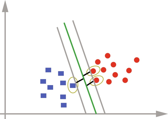
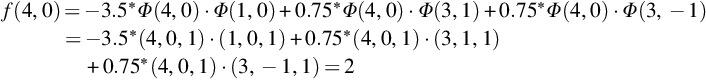
There can be many hyperplanes that will separate the data points. The hyperplane can be chosen as the optimal hyperplane if it has a maximal margin, i.e., the distance d − and d + is maximum. Fig. 15 shows the selection of optimal hyperplane.
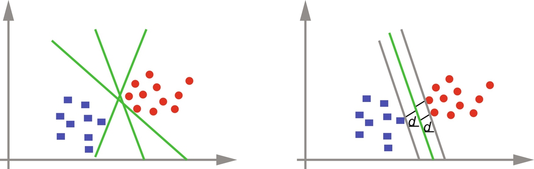
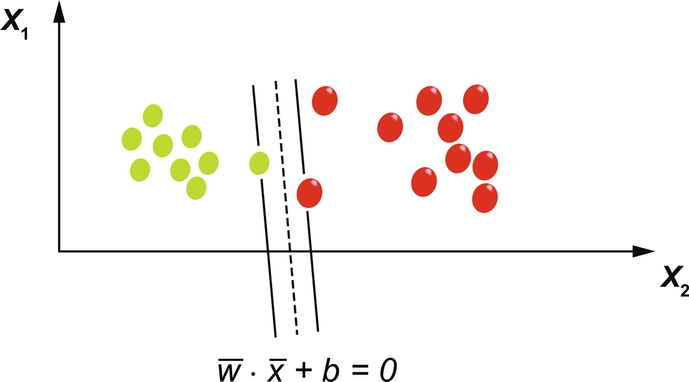
The maximal hyperplane is represented using only those training samples on which the margin depends. These samples are called as support vectors. Fig. 16 shows the support vectors that define the maximal hyperplane.
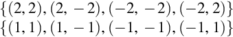
The following example would explain the linear SVM by considering a two-dimensional vector model. For an eight-sample dataset, the first set is positive labeled, while the other is a negative one:
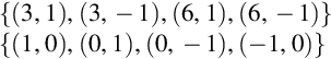
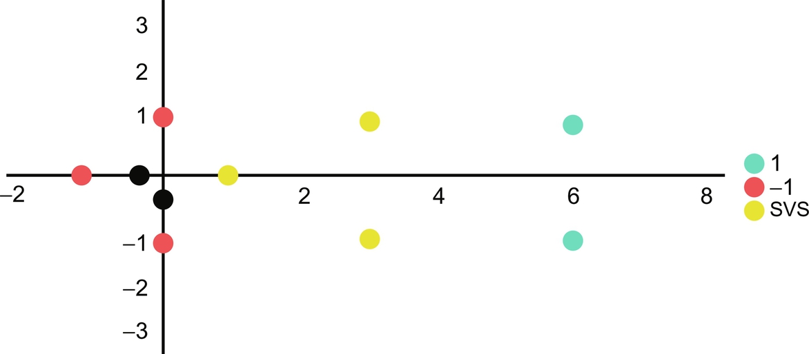
Fig. 17 shows the projection of the above example in a vector space.
As it is clear that the data can be separated, a linear SVM would be the best choice. After inspecting one can easily identify that the hyperplane can be drawn using three support vectors as in Fig. 18. The below equations are used to build the model
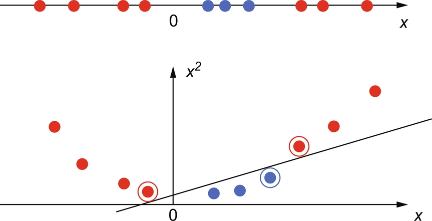
If V1 = (1,0), then Φ(V1) = (1,0,1) by adding 1 as a bias. Dot product of the data points gives us:
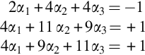
The solution to this system of equations is α1 = − 3.5, α2 = 0.75, and α3 = 0.75.
To obtain the hyperplane, use the below formula:
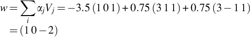
The final hyperplane with the augmented bias which separates the given dataset is y = w*x + b having values as w = (1,0) and bias b = − 2.
Now to check to which class data (1,1) belongs:
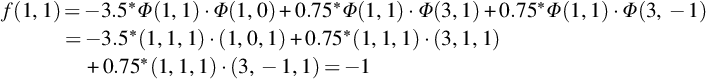
As the value is negative, it belongs to class − 1.
Similarly, to check which class data (4,0) belongs:
As the value is positive, it belongs to class + 1.
There are two types of linear SVM explained in the following section.
6.3.2 Hard Margin Classifier
Hard margin SVM is a strict form of SVM where all samples have to fulfill the marginal condition. When the dataset is free of errors (noise or outliers), the hard margin classifier works as required. In the presence of errors the margin separating the classes will be small or the hard margin SVM may fail. Fig. 19 shows a hard margin classifier.
6.3.3 Soft Margin Classifier
The real-time data on which the machine learning algorithms are applied have noise in them. It is practically impossible to separate the data with a hyperplane. One way to handle this is to relax the constraint of having the maximal margin for the line that separates the classes. This way of relaxing the constraint is known as soft margin classifier. The relaxation allows some point to violate the separating line and be on the other side. Slack variables are some additional coefficients that are introduced in order to make space in each dimension. The complexity of the model increases when more parameters are used to fit the model to the data provided.
The goal of a soft margin classifier is to maximize the margin, while also minimizing the sum of slacks, i.e., to reduce the number of outliers in each group. Fig. 20 shows a vector space of a soft margin classifier.
6.3.4 Nonlinear SVM
Until now a strong assumption was made about the linearity of data. But in practical many datasets cannot be separated linearly. So the assumption that the data is linear is unrealistic. But the linearity of an SVM can be extended to nonlinear SVM by applying a well-known kernel functions or kernel tricks.
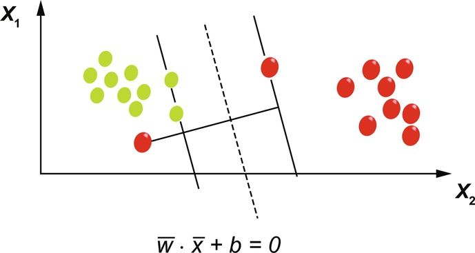
Consider a one-dimensional case as shown in Fig. 21. The dataset cannot be linearly separated. This problem is solved by mapping the data onto a higher dimensional space and then to use a linear classifier in the newly projected higher dimensional space. Fig. 21 also shows how a higher dimension can linearly separate the nonlinear data by using a quadratic function to map the data into two dimensions. This way of projecting data into a higher dimensional space is called “kernel trick.” The kernel trick exploits the mathematics to project the linearly inseparable data to a linearly separable data.
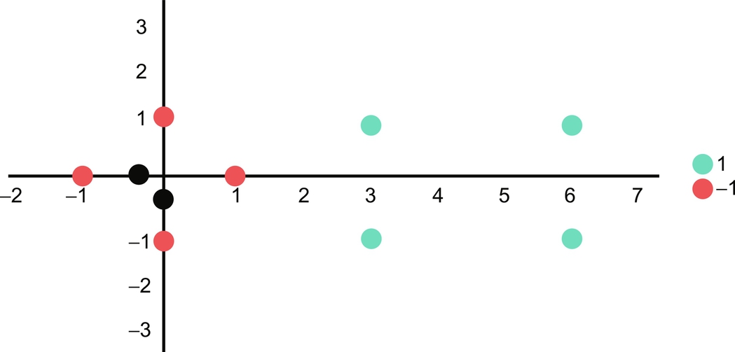
The following is an example to explain a nonlinear SVM:
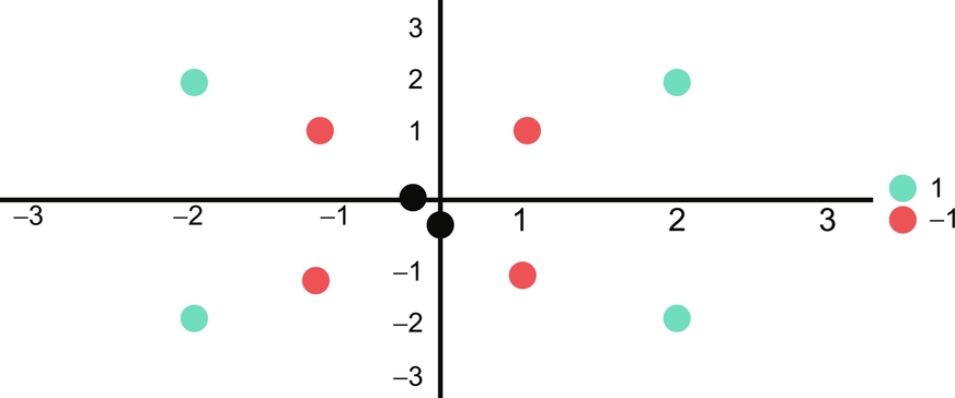
Given below are the two sets of data: the first one representing the positive label, while the second is a negative labeled one:
Projected in vector space looks as in Fig. 22 and clearly indicates that it cannot be linearly separated. Now we will use a transformation function.
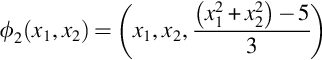
The values are converted based on the below mentioned function:
If x12 + x22 > 2, then ϕ1(x1, x2) = (4 − x2 + | x1 − x2 |, 4 − x1 +| x1 − x2 | )
Otherwise ϕ1(x1, x2) = (x1, x2)
Based on the above transformation the data points get converted as below:
Positive sets:
Negative sets:

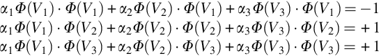
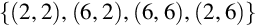
The example of the above data is projected as in Fig. 23 and two support vectors are clearly identified.
The vectors are now used to solve for α1 and α2.
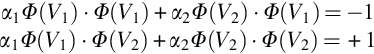
And computing the dot products results in as below:
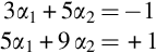
The above equation when solved gives values for the coefficients as α1 = − 7 and α2 = 4 and the hyperplane equation as y = wx + b, w = (1,1) and b = − 3 (b is bias).
To classify the (4,5) dataset into its class:

As value is negative, it belongs to class − 1.
Similarly it is not always possible to solve the nonlinearity problem with same number of dimension. At that time it may be required to project them into different planes using equation as below:
7 Clustering Algorithms
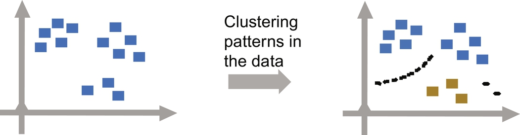
Clustering is an unsupervised learning mode, to draw inferences from datasets consisting of input data without class label or target values, or for exploratory data analysis to find hidden patterns. It groups data instances that are similar to each other in a cluster and data instances that are very dissimilar from each other into different clusters. Cluster analysis is about forming the clusters or organizing the data such that the intracluster distance is less and intercluster distance is more.
In the recent years, due to rapid increase and accessibility of web resources and documents, text clustering has become a significant area of research. Applications of cluster analysis could be gene sequence study, market research, or object recognition in an image, medicine, psychology, sociology, marketing, biology, insurance, archeology, libraries, etc. For example, if a mobile cell phone company wants to optimize the locations where they have to build the towers, machine learning is used to recommend and approximate the number of users relying on their towers. As a phone can connect to only one tower at a time, the team uses clustering algorithms to design the best placement of cell towers to optimize signal reception for groups, or clusters, of their customers.
Popular algorithms to prepare clusters include k-means and k-medoids, hierarchical clustering, hidden Markov models, self-organizing maps, and fuzzy c-means clustering. A diagrammatic representation of sample clustering is seen in Fig. 24.
In a partitional clustering, a set of data objects is divided into nonoverlapping subsets (clusters) such that each data object is exactly one subset. k-means clustering is a partitional clustering algorithm. Hierarchical clustering is a set of nested clusters that are organized in the form of a tree. Divisive and agglomerative clustering are the two types of hierarchical clustering.
7.1 k-Means Clustering
k-means is a clustering algorithm, where a set of data points D from a chosen dataset are partitioned into k number of clusters. Each cluster has a cluster center, called centroid. Value of k is to be specified by the user. Fig. 25 represents an example showing step-by-step clustering process.
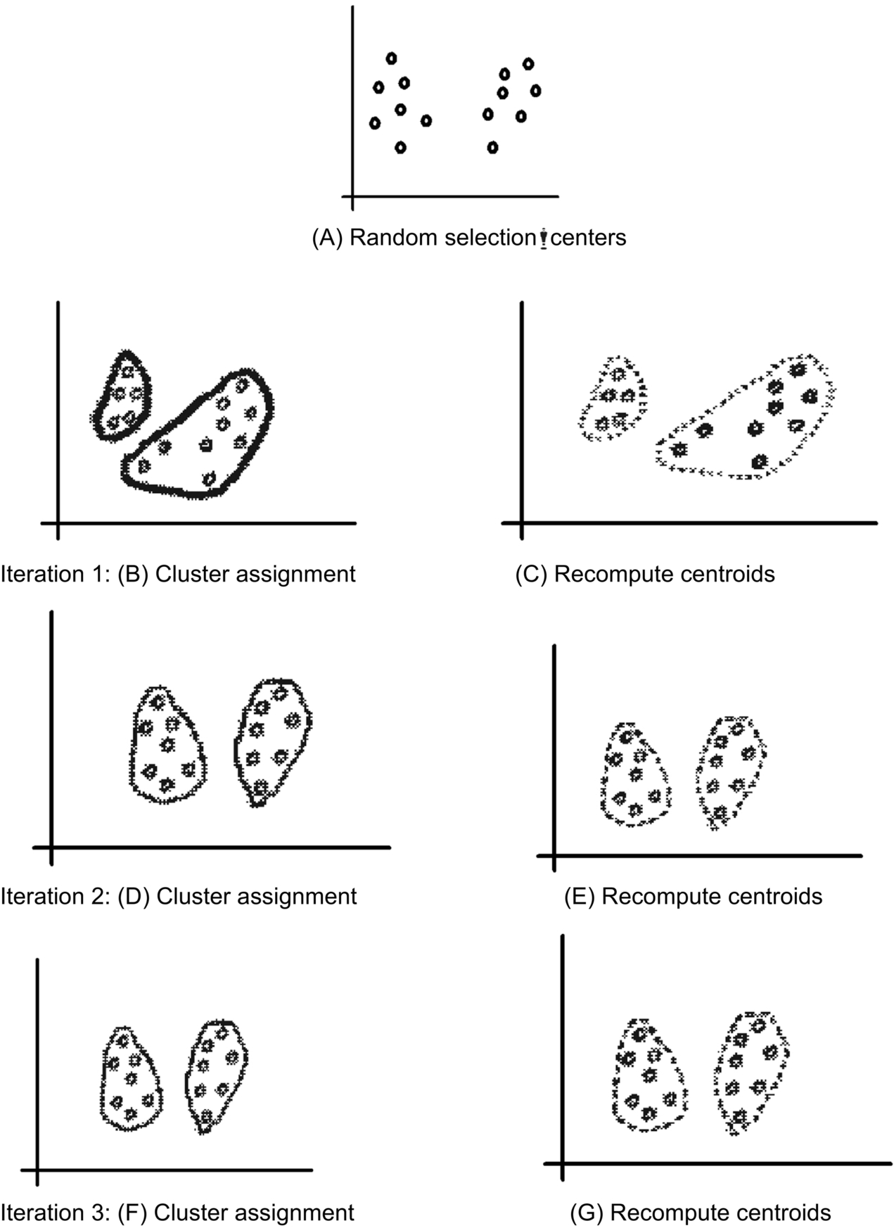
The steps in which k-means clustering algorithm works are as follow:
- Step 1: Choose k data points (seed value) randomly, to be the initial centroid, cluster centers.
- Step 2: Assign each data point to the closest centroid.
- Step 3: Recompute the centroids using the new cluster memberships.
- Step 4: Check if the union is met, otherwise go back to step 2.
Advantage of k-means algorithm: This algorithm is simple, easy to understand, and implement. It has a time complexity of O(tkn), where n is the number of data points, k is the number of clusters, and t is the number of iterations. As the values of k and t are small, k-means clustering algorithm is considered to be linear.
Disadvantage of k-means algorithm: k-means algorithms can be used only if the “k” value is well defined in the beginning. The algorithm may not perform well with outliers. Outliers could be an error in the dataset or a special data point with unusual value.
7.2 Hierarchical Clustering
A hierarchical clustering algorithm works on the concept of grouping data objects into a hierarchy of “tree” of clusters. Hierarchical clustering is divided into agglomerative or divisive clustering, depending on whether the hierarchical decomposition is formed in a bottom-up (merging) or top-down (splitting) approach. In agglomerative clustering partitions are visualized using a tree structure called dendrogram. Height of the dendrogram is to be decided by the data analyst or a researcher working on clustering. Divisive clustering, a top-down approach, works on the assumption that all the feature vectors form a single set and then hierarchically go on dividing this group into different sets. A sample flow of agglomerative and divisive clustering is shown in Fig. 26.
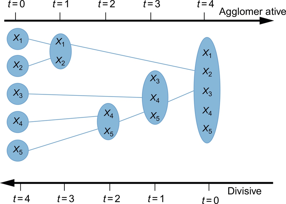
In both agglomerative and divisive hierarchical clustering, users need to specify the desired number of clusters as a termination condition.
The steps for forming agglomerative (bottom-up) clustering are:
- Step 1: Start by considering each data point as its own singleton cluster.
- Step 2: After each iteration of calculating Euclidean distance, merge two clusters with minimum distance.
- Step 3: Stop when there is a single cluster of all examples, else go to step 2.
The steps to form divisive (top-down) clustering are:
- Step 1: Start with all data points in the cluster.
- Step 2: After each iteration, remove the “outsiders” from the least cohesive cluster.
- Step 3: Stop when each example is in its own singleton cluster, else go to step 2.
8 Applications
Machine learning techniques are being applied in a wide range of applications in order to solve number of fascinating problems.
- 1. Contextualized experience goes beyond simple personalization, such as knowing where the user is or what they are doing at a certain point in time. An abundance of available data enables improved features and better machine learning models to be created, generating higher levels of performance and predictability, which ultimately leads to an improved user experience.
- 2. With the rapid increase in devices and applications connected to the Internet of Things, the sheer volume of data being generated will continue to grow at an incredible rate. It is simply not possible for humans to analyze and understand such quantities of data manually. Machine learning is helping to aggregate all of this data from countless sources and touch points to deliver powerful insights, spot actionable trends, and uncover user behavior patterns.
- 3. Retail buyers are being fed live inventory updates and in many cases enabling the autoreplenishment of stock as historical data predict the future stock-level requirements and sales patterns.
- 4. Healthcare providers are receiving live updates from patients connected to a variety of devices and again, through machine learning of historical data, are predicting potential issues and making key decisions that are helping save lives.
- 5. Financial service providers are pin pointing potential instances of fraud, evaluating credit worthiness of applicants, generating sales and marketing campaigns, and performing risk analysis, all with the help of machine learning and AI-powered software and interfaces.
- 6. Statistical techniques may mechanically create segments and groups that make sense on the data.
- 7. Data analyst uses machine learning techniques to identify the key influencers on profitability.
9 Conclusion
Today, machine learning has progressed from research to mainstream and is a motivational drive in an era of innovation. Today, industries need to think on how machine learning can help them in creating a competitive advantage. Few may use data to spot the trends in performance of employees or their market products. This will help them to predict and prepare for future policies and outcomes. Others may use learning models to personalize their inventory, creating a better user experience and promoting an increased level of involvement with their existing and potential customers.
As the level of accessible data continues to grow, and the cost of storing and maintaining it continues to drop day by day, more and more machine learning solutions hosting pretrained models-as-a-service are making it easier and more affordable for organizations to take advantage. From a development point of view, this is enabling the quick movement of application prototypes into production, which is exponentially increasing the growth of new applications and startups that are now entering and disrupting most markets and industries out there.
9.1 Challenges and Opportunities
Previously, only a few big companies had access to the quality and size of datasets, required to train production-level AI. However, now startups and even individual researchers are coming up with their own clever ways of collecting training data in cost-effective ways. With the increase in collected data and connectivity among devices and applications comes the challenge of addressing data leaks and security breaches which may lead to personal information finding its way into the wrong hands and applications.