Expanded Uses for BGP
Abstract
In this chapter, you will learn more about the newer features of Border Gateway Protocol (BGP). BGP, as we have seen, is the main way that information about routes gets around the global public Internet. Once used exclusively for spreading “routing about routing” information, BGP now forms the basis for many advanced capabilities.
We will examine the two advantages BGP enjoys when used for new purposes. First, BGP was designed to be extensible, so new features can be added without inventing a completely new protocol. In most cases, if a BGP peer does not know how to parse and use a certain type of update inside a network layer reachability information (NLRI) update, the receiver can simply ignore it (although in many cases, it will still have to pass the information on to other peers). Second, BGP crosses routing domain (Autonomous System or AS) boundaries with ease, something it was designed to do.
You will learn how to configure BGP for one new feature in the Illustrated Network, in this case how to use BGP to distribute interior gateway protocol (IGP) metrics outside an AS boundary.
Keywords
Border Gateway Protocol (BGP); network layer reachability information (NLRI); interior gateway protocol (IGP); Optimal Route Reflection (ORR); VPN; LAN; TCP/UDP
In this chapter, you will learn more about the newer features of Border Gateway Protocol (BGP). BGP, as we have seen, is the main way that information about routes gets around the global public Internet. Once used exclusively for spreading “routing about routing” information, BGP now forms the basis for many advanced capabilities.
We will examine the two advantages BGP enjoys when used for new purposes. First, BGP was designed to be extensible, so new features can be added without inventing a completely new protocol. In most cases, if a BGP peer does not know how to parse and use a certain type of update inside a network layer reachability information (NLRI) update, the receiver can simply ignore it (although in many cases, it will still have to pass the information on to other peers). Second, BGP crosses routing domain (Autonomous System or AS) boundaries with ease, something it was designed to do.
You will learn how to configure BGP for one new feature in the Illustrated Network, in this case how to use BGP to distribute interior gateway protocol (IGP) metrics outside an AS boundary.
Introduction
This chapter began as a series of notes I called “new tricks for BGP.” BGP started as an infrastructure protocol and first evolved to a basic connectivity method and now to an underlay for advanced service networks. An “underlay” is a basic network protocol used to support the features of a protocol or service running as an “overlay” so that the entire protocol does have to be duplicated. Later on, we’ll see a case where a Layer 3 routing network underlay supports a virtual Layer 2 LAN-type network overlay.
BGP emerged in 1989 as the need to share information across independent routing domains became necessary. In fact, BGP has become so common as the basis for new capabilities on the Internet that this chapter has had to exclude many of them and concentrate on only a few.
Many services on the Internet are moving to BGP:
We will also investigate some of the newer uses of BGP in the data center, a role that was never imagined not so long ago. These applications include:
BGP Labeled-Unicast-based Egress Peering Engineering (BGP-LU-based EPE)
Some of these are beyond the scope of an introductory text. Others, armed with a basic understanding of BGP message formats and procedures, we can explore in detail.
In particular, we will explore four main areas for uses of BGP:
We’ll close with a quick look at the statements needed on the Illustrated Network to implement BGP-LS.
Optimal Route Reflection (ORR)
When a routing domain uses BGP, scaling the peering sessions required to establish the Routing Information Base (RIB) can be done using a BGP router reflector (RR) instead of a fully meshed IBGP session. Instead of sharing information with every router running iBGP in the routing domain, the RR client routers peer only with the RR. The RR decides what the “best path” to each destination is and the RR then distributes this information to each and every router in the area covered by this particular RR.
The whole point of iBGP is to distribute information about AS “exit points” for certain IP prefixes, such as the location of provider edge (PE) routers used to reach a destination. Router reflectors have clients running iBGP, and even eBGP if they are on the packet forwarding path and can reach BGP AS border routers (ASBRs) in other routing domains. All the clients and the RR form a collection called a “cluster” that is identified with a 32-bit number similar to an IPv4 address. The cluster ID is a cumulative, non-transitive attribute of BGP. Every RR prepends their local cluster ID to a “cluster list” to avoid routing loops.
Route reflection cuts down on the number of peering sessions needed for iBGP and lets the AS scale higher than without route reflection. For example, mesh iBGP peering of 10 routers requires 90 TCP sessions to be established and maintained, along with their associated database (routing information base or RIB). The formula is N=R×(R−1), where R is the number of routers in the AS running iBGP and N is the number of peering sessions required. Now, there are R×(R−1)/2 links between these 10 routers (45 links), but each endpoint of the point-to-point link has to maintain the session information and RIB for that peer. For 100 routers, N is a staggering 9900!
The nice thing about RR devices is that they can be used with eBGP peers and iBGP peers that are not part of an RR clusters. How does this work? Route reflectors, which are technically “servers,” propagate routes in the domain with three main rules:
• If the route is received from a non-client peer, then the RR reflects the route to its clients only and all eBGP peers.
• If the route comes from a client peer, reflect that to all non-client peers as well as client peers, except the originator of the information. Also, reflect this information to eBGP peers.
• If a route is received from an eBGP peer, reflect this information to all client and non-client peers as well as other eBGP peers.
“Regular” Route Reflection
A generic use of RR devices is shown in Figure 17.1.
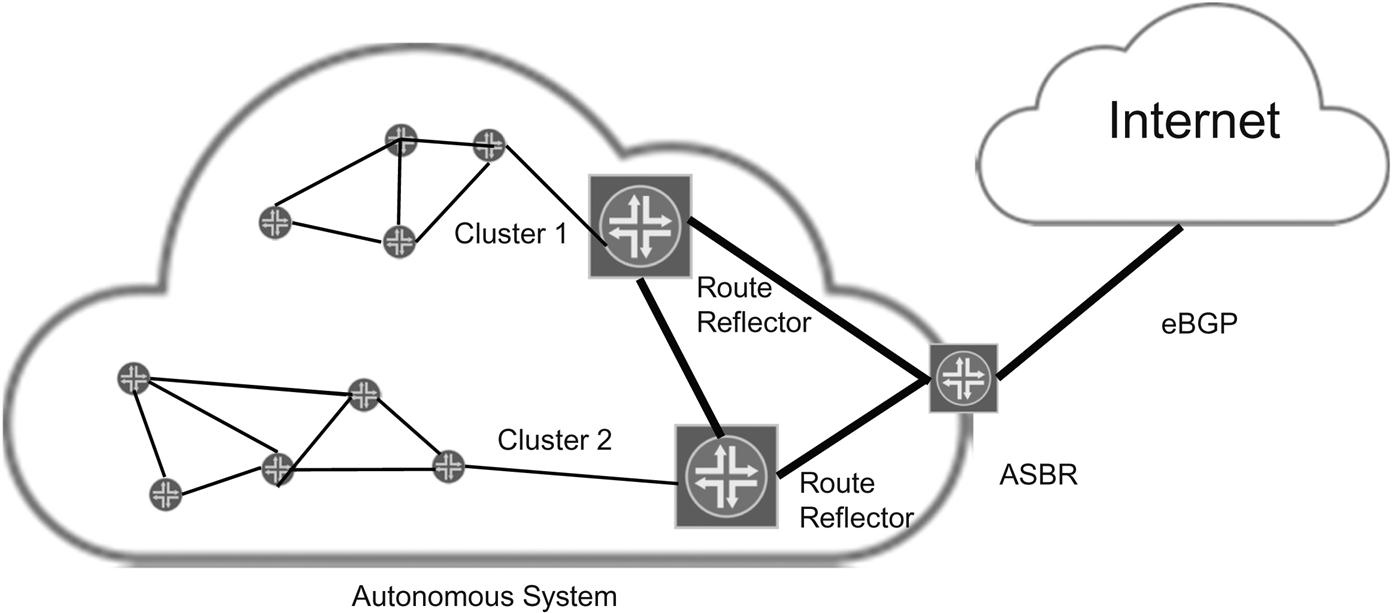
With an RR running on one of the 10 routers, the same number of peering sessions is only 18 (if the RR is not also a forwarding point). In most cases, there is more than one RR for a cluster, because the RR device is a single point of failure. But it is not necessary to explain all of the quirks of route reflection to understand ORR.
It is enough to note that a routing domain can have many RR routers, and that these can be dedicated routers that only exist to reflect routes and paths to other devices, or the RRs can also be used to route “regular” traffic as well as reflect routes. The issue depends on many factors, including the power of the routers, the number of reflected routes, the need for redundancy (high availability), and the extent of the sphere covered by the RR.
For this section, one aspect of RR operation is essential. The RR device chooses the best path from its own perspective (usually the active route) and it is only this route that is advertised to the clients of the particular RR. In other words, the choice of the exit point for the RR and all its clients in the one that is best for the RR, not necessarily all of the clients that receive the reflected information.
As RFC4456 on BGP RRs puts it, because the IGP cost metric to a given point in the network varies from router to router “the route reflection approach may not yield the same route selection result as that if the full IBGP mesh approach.” The impact of this practice is that it can ruin attempts to impose “hot potato” routing in the routing domain. Hot potato routing tries to direct traffic to the “best” AS exit point in cases where no higher priority routing policy demands another exit be used.
But in many cases it would be better for the RR to pick the best path from the client’s perspective. That route is then selected to be reflected to the client. This matching of iBGP mesh best path with RR best path can be accomplished by placing RR devices outside of the forwarding path, often gathered in the core of a large ISP network.
However, this practice leads to the drawback mentioned above: when the RR learns of a route from multiple devices, it relies on the IGP metric to select the best paths to advertise to the clients. This will often be the exit point closest to the RR and not necessarily the client router. There are workarounds for this, but ORR solves the problem directly.
ORR Considered
Let’s look at a case where ORR is needed. Figure 17.2 shows a route reflector getting a network layer reachability information (NLRI) message about network 10.7.7/24 from different PE routers. All three—PE1, PE2, and PE3—can reach 10.7.7/24. The RR knows both PE2 and PE3 can reach 10.7.7/24, but because of the IGP metric, the route through PE3 becomes the active router and PE2 a known path, but inactive. So because the cost metric on the link to PE3 is less than the cost metric to PE1 or PE2 (in spite of the cost between them), PE1 is told by the RR to reach 10.7.7/24 through PE3 instead of PE2, which is clearly not the “best” path.
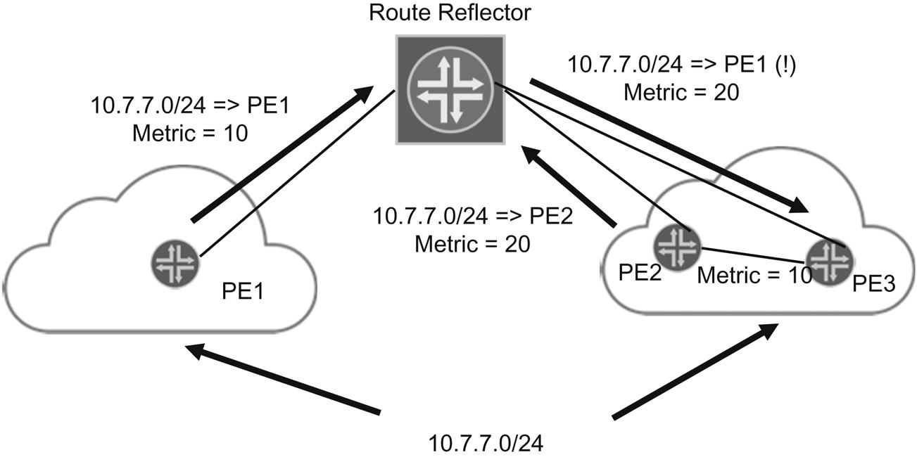
With ORR, the router reflector will reflect the proper path from PE2 to PE1, as expected from the topology. To accomplish this, ORR adds two modifications to the RR algorithm and “rules” to find the best path. ORR devices can implement one or both of these modifications as needed to obtain the result desired. The nice things about these modifications is that only the RR devices and not the client routers need to be modified for the new software features of ORR.
The two modifications are referred to the draft as IGP-based best path selection and policy-based best path selection.
In IGP-based selection, the RR is assigned a “virtual” IGP location and metrics. This virtual location can be specified per RR, per peer group, or per particular peer. When considering the best path to a given destination, the RR can now use the details of the virtual location in the network inside of the “IGP location” to consider the best path. Interestingly enough, the draft does not contain any details as to how the route selection calculation is changed to complete the IGP metric adjustments needed. For details, please see the ORR Internet draft.
In policy-based selection, an additional routing policy is applied to the information received by RR clients (and perhaps other routers). Because it is an established policy, this approach can be good for mandating dedicated exit points for certain destinations. Because of potential interactions when both modifications are used, the policy is always applied first before any other best path selection, which might include IGP-based modifications, takes place. So whatever the policy, the route information is still subject to normal RR route selection rules and even IGP-based ORR. This makes the two modifications very flexible to implement and consistent in result.
Now, ORR does not really add much to BGP or route reflection itself. What can BGP do to help other types of services besides BGP? Let’s take a look at how BGP works with flow specification.
BGP and Flow Specification
A flow is defined as group of fields in IP and TCP/UDP headers that share common values. This group is called an “n-tuple” and is usually implemented as a set of matching criteria rules in a routing policy. For example, a packet can be examined to evaluate the source and destination network prefixes, the protocol carried, or TCP/UDP port numbers.
An individual packet belongs to the defined flow if these headers fields match every specified value (which might include ranges) in the n-tuple. After a flow spec is made, there are also a set of defined “actions” that determine what the router should do with the corresponding packets that make up the flow. These actions might include changing the next-hop destination, counting the packets, classifying them for class of service (CoS) purposes, or all of these at the same time.
Although this deep examination of packet headers is only now becoming the normal processing procedure on a network node, routers have done more than merely forward traffic since they were first developed. As RFC5572 on the dissemination of flow specification rules notes, routers have long been able to “classify, shape, rate limit, filter, or redirect packets” based on policies defined on the router. Routine use of flow specs is a natural evolution of these capabilities. Only a few years ago, it was a very real burden on the processing power of the router to look at packet headers as the router struggled to keep up with every-increasing line rate of input ports. These inputs often few low-speed output ports, requiring a lot of memory dedicated to output packet queues (memory dedicated to input and output ports are called “buffers”).
Using BGP with flow specification has been around for a while, at least since 2009 with RFC5575. However, it is only in the past few years that ISP and other Internet-related groups have applied BGP flow specification (RFC5575) to traffic diversion to react to distributed denial-of-service attacks. This is the aspect of BGP and flow specs that we will explore in this section.
Why should using BGP with a flow specification be so special? Because BGP goes everywhere… iBGP goes everywhere inside the AS, and eBGP goes outside. It should be noted that the implementation of eBGP flow specs (i.e., outside the AS), requires the agreement on its use by the organizations administering the ASs. Without such cooperation, it makes little sense to send flow spec information outside the iBGP sphere.
In fact, the power of BGP flow specs is greatest precisely when this technique is applied among more than one organizational AS or routing domain. Consider the case where BGP flow specs can be used to blunt the force of a distributed denial-of-service (DDoS) attack on a victim, usually a large web site or other central collection of servers.
BGP and DDoS
The basics of a DDoS attack is shown in Figure 17.3. There is nothing unusual about the figure: clients are attached to the global public Internet on the left, and the server reside in an enterprise network or large data center on the right. In the middle is the customer’s service provider network, although most of the customer site protection is provided by firewall or intrusion detection systems on the server side, not the network side. As a result, attacks are not easily deflected until they have compromised the service provider networks as well as the customer site. This is one problem that BGP flow specs can solve.

The DDoS attack begins when a number of software bundles are placed on otherwise innocent client computers attached to the Internet. This software often hides inside otherwise innocent packages of upgraded freeware, drivers, shared files (often of copyrighted material), and so on. Normally, hacking attacks would be easy to deflect by the site firewalls, as shown by the lower arrow, because the original of the attack soon becomes well known.
However, the power of a DDoS attack is twofold: the attack is launched from many places (often distributed among thousands of infected “bots” that are triggered all at the same time) and that attack masquerades as simply a large number of visits to particular server site. However, as shown in the figure, these bot-compromised systems can quickly overwhelm service provider network capacity as the traffic concentrated as it moves closer and closer to the target victim site. Once at the site, the DDoS traffic, which is otherwise indistinguishable from regular client queries, also overwhelms the inline security devices such as the firewall(s) and intrusion prevention systems. When unchecked, the DDoS traffic saturates the target service or application at the victim and, as a result, denies service to the legitimate users of the site.
How does BGP help this DDoS situation? In one of two ways. The first way is shown in Figure 17.4. In this case, the victim data center or enterprise can use BGP flow spec updates to initiate a BGP announcement to temporarily “black hole” (send to the bit bucket) the traffic flow that characterizes the DDoS attack. It might not be obvious that a DDoS traffic stream contains enough common header fields to define a flow, but if the attack is to be effective, the traffic generated by the bots must be targeted as precisely as possible.

Once these BGP updates reach the service provider routers, they establish a remotely triggered black hole (RTBH) at the peer service provider edge (because this is where the DDoS traffic enters and leaves the network). These BGP updates have the next-hop set to a preset black hole route. As a result, the destination RTBH discards all traffic to the victim until the flow ceases for a certain amount of time and normal routing to the victim resumes.
Now, many service providers might be nervous about letting their customers set next hops in their core network, whether on the edge or not. So there is another way to halt the DDoS attack flow with BGP. In this case, the BGP next-hop updates for the DDoS victim are detected and triggered by the service provider. This is shown in Figure 17.5. The only difference is that in this second case, the victim might not even be aware that the DDoS attack has taken place, unless some reporting mechanism is in place (and usually is).

Note that in both cases, not only with DDoS attacks, but with other types of hacker activity, these attacks can be deflected by using BGP with RTBH next hops. The major difference is who know about the attack first and who issues the proper BGP updates to start and end the black hole.
BGP Flow Spec Details
How does BGP perform this flow spec magic? Through NLRIs, of course. RFC5565 established an Address Family Identifier (AFI) and Subsequent AFI (SAFI) values for flow specs and these were extended to IPv6 later. The AFI/SAFI values are:
In these NLRIs, the routing “prefix” contains the destination and source IP address, as well as the protocol and port that applies to the matching rule. For example, the advertised information could be something like <dest=10.0.1/24 (more specific forms possible), srce=* (any), protocol=6 (TCP), port=80 (html/web)>. BGP routers then understand flow spec NLRIs can implement the flow spec rules any way they like (within limits: there is an order that the flow spec rules must be applied to prevent interpretation conflicts). For example, Juniper Networks devices will keep flow spec routes in a separate table (inetflow.0) and apply the contents of this table as an ingress forwarding table filter. In Juniper Network’s implementation, the flow spec routes are always validated against unicast routing information or through the devices’ routing policies.
Flow specs can match on the following:
• Destination and source prefix
• IP protocol such as TCP, UDP, ICMP, and so on
• Destination or source port (TCP or UDP)
• Fragmentation values (do not fragment, last fragment, more fragments, and so on).
Implementation often adds several other parameters to these fields. For example, some Juniper Networks routers allow the setting of additional match parameters such as:
• Bandwidth: The number of packet-per-second of the matched traffic type the device will accept
• Burst: The number of packets of the matched type that the router allows during a burst
• Priority: specifies are priority level for the matched packet (such as “low”)
• Recovery time: The number of second that must elapse before the matched flow is considered revered from the attack
• Bypass the aggregate policer: The DDoS protection will bypass any aggregate policer configured for the protocol group (for details, see Juniper Networks technical documentation)
• Disable lice card (FPC) or routing engine policers: Another Juniper-Network-specific operation
• Disable logging: Do not log the DDoS event (DDoS attacks can overwhelm device logging capabilities).
This is not even an exhaustive list. All of these parameters are configured optionally and have default values and actions. Other parameters include line card specifics as well as bandwidth and burst scaling percentages. All in all, Juniper Networks routers allow 12 different additional parameters for DDoS protection, all under a ddos-protection stanza in the configuration.
The actions that a flow spec can take are defined using Extended Communities in BGP:
• 0x8006: traffic rate (a rate value of 0 discards all traffic in the flow)
• 0x8007: traffic action (for instance, sample the flow periodically)
• 0x8008: redirect the flow to a certain routing instance
• 0x8009: mark the traffic (e.g., with a certain DSCP value).
When it comes to DDoS protection, many implementations simply silently discard the traffic (the whole RTBH concept). After all, it makes little sense to add processing complexity to a network currently under DDoS attack.
Although flow spec use in BGP is very flexible, the main purpose of these NLRIs is to make the distribution of traffic filter lists to routers more or less automatic during DDoS attacks. Routers that understand these NLRIs can drop traffic flows based on the packet and TCP/UDP header fields referenced by the AFI/SAFI. Each router can do this independently, but it makes a lot of sense to coordinate actions when routers are struggled under a DDoS attack in the first place. So a central platform can build filter rules to drop the harmful traffic and distribute these in advertisements to BGP peers.
It is often problematic to use IP prefixes as the basis for flow spec traffic diversion. This is a large hammer to use for a problem that is often best addressed using a more focused method. So there is a way of using the redirect action to perform a kind of “surgical diversion” of suspect traffic to a “scrubbing center” where further action can be taken. This mitigation can even include the reinjection of traffic once the central location has decided what to do.
In several implementations, it makes a lot of sense to make central point of coordination the route reflector.
In summary, here are the benefits of using BGP flow specs to address the issue of DDoS attacks, with or without surgical diversion:
• The filtering rules are “piggybacked” onto regular BGP NLRI distribution, which is common inside (iBGP) and outside (eBGP) routing domains.
• The new address family (AFI/SAFI values) separates filtering information from pure routing information (and in most implementation is kept in a separate “flow spec” table).
• The method provides a good tool to react to DDoS attacks quickly and automatically, saving valuable time between attack detection and mitigation efforts.
BGP in the Very Large Data Center
One of the most startling things about the new aspects of BGP is its use in places where BGP was seldom found not too long ago. But new Internet drafts propose the use of BGP in “large-scale” data centers… and they mean VERY large: places with “hundreds of thousands of servers.” Nevertheless, BGP in the data center is worth discussing, not only because the role that BGP would play in a data center is not obvious, but because many things that apply to extreme cases in networking end up being useful in more routine environments.
Data Centers as CLOS Networks
A lot of concepts and network architecture are taken from the old Public Switched Telephone Network (PSTN) in the United States. Often the connection between these original voice network innovations and their later implementation in, e.g., a modern data center is not obvious. Let’s look at how something called a CLOS network is used in a data center and how BPG often plays a role as well.
At first it might seem odd that the meta-routing protocol (“routing about routing”) like BGP could apply in the tight, closed world of the data center. However, the challenge of networking is often keeping apart things that naturally belong together and bringing together things that naturally want to stay apart. For instance, a Layer 2 network like a LAN connected by switches or bridges naturally forms one big network while a Layer 3 network connected by routers naturally forms many networks, but all interconnected at Layer 3.
Let’s see how this all comes together with BGP. Many data center designs are based on a PSTN architecture called a CLOS network or folded CLOS network. Why? Well, the Clos concept worked well for the voice network, so it made no sense to reinvent the wheel when it was time to invent an architecture for large-scale data centers.
What is it about large-scale data centers that make CLOS networks such a good fit?
To see that, we need a bit of history. Once a telephone became popular among “subscribers” (as customers for the voice service were known) the question of how to pay for the service came into play as well. Early customers rebelled at flat-rate services, where subscribers paid a fixed amount per month whether they called anyone or not, and there weren’t that many people to call then at all. So the leading payment model became metered services, a kind of pay-as-you-go service that recorded and billed based on the calls you made (incoming calls were free to encourage people to get phones).
But there were two situations that could cut down on telephone company revenues. It is good to remember that if you called someone, a connection path through the network had to be found and set up before the phone would ring at the other end of the line. In some cases, all this work was done only to find that the other person was already on a call. In that case, there was nothing to do but give the caller a “busy signal” and hope they would call back later (they usually did).
The other case was a bit trickier. In that case, the connection attempt was blocked along the path because there was no circuit path available between telephone switches. Eventually, the caller would receive a “fast busy” tone to indicate this lack of resources in the network. If this condition happened frequently enough, it could severely impact the revenues of the telephone company. If only there was a way to maximize the resources of a given network so that there were many multiple paths through the network to route connections.
This is where Charles Clos comes in. Charles Clos worked at Bell Labs, the R&D arm of the AT&T Bell System, the largest telephone network in the United States and the world (in 1970, AT&T had a staggering 1 million employees). In an article published in 1953 in Bell Labs Technical Journal, Clos explored the mathematics behind a type of multi-stage “crossbar” switch that allowed graceful scaling of larger and larger capacity switches (i.e., inputs and outputs).
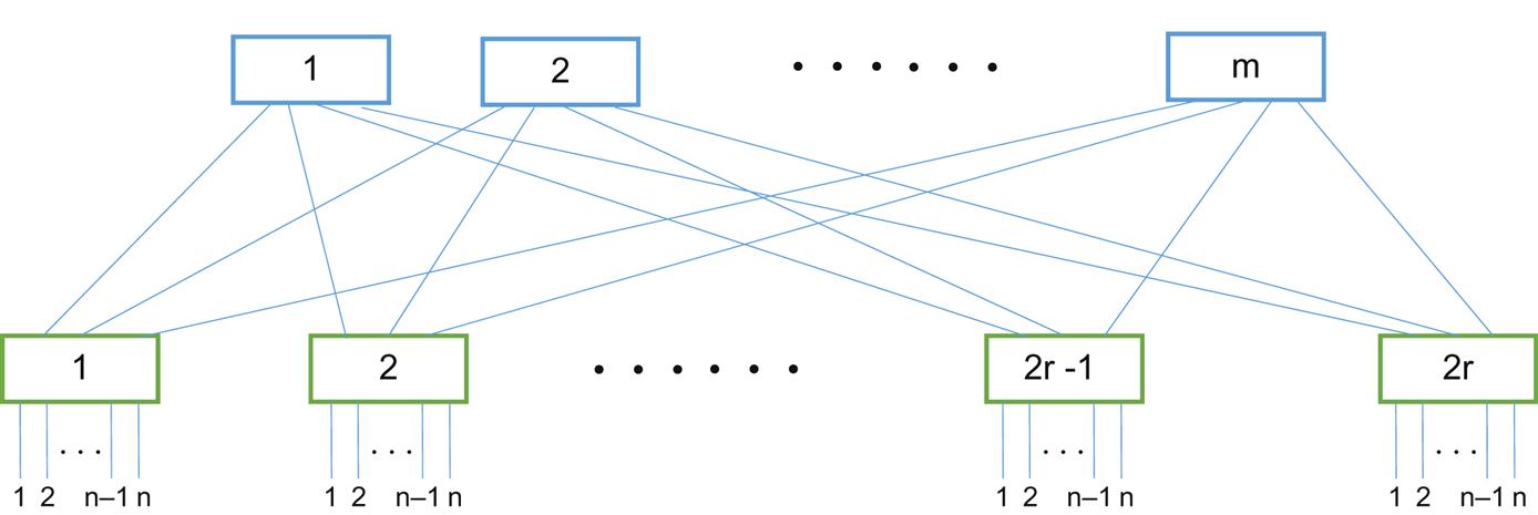
CLOS networks consist of three stages: the ingress stage, the middle stage, and the egress stage. Each stage is made up of a number of “switch points” (crossbars) to route calls (or any type of traffic) from an input port to an output port. The characteristics of the CLOS network are defined by three integer parameters: n, m, and r. The number n represents the number of inputs that feed the r ingress stages, while the number m represents that number of outputs for each switch stage.
Clos’s paper showed that if the number of stage outputs (m) was greater or equal than twice the number of inputs (n) minus 1, there would always be a path through the network from input to output:

That is, the switch would be non-blocking. Scaling would be provided not necessarily by increasing the values of m and n, although that was possible, but by adjusting the value of r, the number of inputs and outputs in each individual switching element.
The CLOS network concept can be made much clearer by showing the relationship of the numbers in Figure 17.6. Note that the gross number of inputs and outputs (n) is not the same as the number of stage outputs (m) or the way the ports are packaged in a stage element (r).

Let’s see if you’ve been paying attention. Is the folded CLOS network shown in Figure 17.1 blocking or non-blocking? The formula is  , and we see in the figure that n=4. Therefore, we need 2×4−1=7 middle stage switches. But there are only 3 shown. (And obviously, if there are only three outputs to the three middle switches, for example, the fourth input from each ingress stage will always be blocked). However, we have an out: the dotted lines indicate that there could be more links and stages than shown in the figure.
Now the attraction of CLOS networks for large-scale data centers becomes obvious. But in the data center, it’s common to represent the CLOS network in a folded form by realizing that the n ports can be connections to the client and server hosts (or their VMs) inside racks in a big data center. To show this, we can just “fold” the CLOS network in the middle, making each input n also a potential output n and making the middle stage a second level on top of the first level ingress stage switches. This folded CLOS network is shown in Figure 17.7.
Now, in a real data center, the top of rack (TOR) switches usually form another level in the network, below the stage shown in the figure. In this architecture, the TOR switches feed the “leafs” of the folder CLOS network, and these leafs are linked by a third level called the spine. In some data centers, the top level can perform gateway functions to other data centers of the Internet, or the spine devices can try to provide this “gateway router” function. Any oversubscription, which is the allowance of ports in excess of the strictly calculated Clos capacity, can be done at the TOR level.
There is no standard definition of the levels or components, leaving each explanation the burden—or freedom—to define its own terms. In this chapter, we’ll use the TOR-Leaf-Spine model and not worry about leaving the data center. (There is a lot of documentation that mentions Tier 1, Tier 2, and Tier 3 devices in the data center, but this terminology is also used for reliability capabilities, so we will not employ it here.)
Layer 2 and Layer 3 in a Folded CLOS Network Data Center
So far, we have taken the concepts of the CLOS network and extended them to data centers. But have we created one big monolithic network or many smaller interconnected networks? As mentioned earlier, the challenge of networking is keeping apart things that naturally belong together and bringing together things that naturally want to stay apart. Which case are we looking at in a big CLOS network data center?
Let’s first examine the consequences of placing each server or host into one giant Layer 2 network, making the data center a LAN connected by switches or bridges. Let’s call this the “Layer 2 data center.” Then we’ll look at making multiple Layer 2 networks in the data center, but connected by routers interconnected at Layer 3. The good news is that there is no single right answer, but the bad news is that at some point scaling issues tend to indicate it would be more efficient to use Layer 3 in the data center, and perhaps even use BGP to further break the data center up into independent routing domains (autonomous systems).
The nice thing about creating a single data-center-wide Layer Lan is that servers (and the services they host) can be as mobile as we like. There is no location implied by a Layer 2 MAC address, so it does not matter which rack, shelf, or slot the endpoint of a connection dwells. But this scheme works best with a limited number of devices and ancillary protocols such as TRILL (Transparent Connection of Lots of Links: RFC6325). Otherwise, at some point scaling issues make bridging convergence a nightmare, broadcast storms might never end, and the sizes of the MAC and ARP tables would be gigantic.
Also, verbose TCP tends to overwhelm larger data centers. Critics of the Layer 2 approach point out the data centers using Layer 2 exclusively are trying to solve a problem that has already been resolved with IP and Layer 3 protocols.
But if we go to Layer 3 for the data center, which routing protocol should be used? It would be nice to use OSPF or IS-IS, but routing database size quickly becomes an issue as the number of Layer 3 devices rises. The leaf-spine-gateway architecture is inherently hierarchical, but both OSPF and IS-IS tend to view hierarchies on their own terms, with continuous areas or levels. Also, traffic engineering, necessary to shift traffic around a spine that is under maintenance, is possible with both IGPs, but this is seldom easy.
Finally, and most tellingly, the data center network needs an EGP such as BGP in any case. If nothing else, the data center routing domain will be separated from any external routing domain. So if at least one BGP AS is needed, why not explore possible roles for multiple ASs in a large data center?
So, in this way of thinking, the large-scale data center should embrace BGP because BGP is extensible, stable, and universally supported.
Data center switch purists might be surprised at this point. But the goal is to make things work, not try to stretch a methodology beyond its limits just to prove a point. To skeptics, we might point out that:
• BGP is not only alive and well, but evolving. And it is the engine of the Internet.
• BGP tends to get very complex when needing complex routing policies, true. But we’ll soon see that there is really no need for complicated policies in a data center, and that what you need is to spread the reachability information around.
• BGP sessions do have to be configured, but that’s true of everything. If BGP can improve your data center fabric performance, it’s always worth doing.
• BGP implementations have been slow to converge because it better to make sure the global public Internet keeps chugging along. But data center BGP can converge as fast as an IGP when adjusted correctly.
• BGP configuration is usually more lines and larger than using an IGP-like OSPF configuration, but the use of widespread network automation to push configurations to devices makes this a small objection.
Use iBGP or eBGP?
BGP, as we have seen, comes in two major packages: internal BGP for use inside an AS routing domain and external BGP for use among AS routing domains. This issue is very important, but most data centers divide their tiered devices up into multiple AS routing domains and run eBGP among them.
Why not iBGP? Using iBGP would require all switches, even the TOR switches, to peer with every other device running Layer 3 in the data center. Of course, the peering burden and overhead can be lessened by using route reflectors, and several major data center schemes propose doing just that.
However, standard BGP route reflection only reflects the “best” route prefix. This makes route reflection very difficult to use with equal-cost multipath (ECMP) schemes, which we definitely want for the large data center. Traditional IGP routing, and basic BGP route reflection, favors the path with the lowest metric “cost” value. If several paths have the same cost, IGPs pick one to use and basically use the rest as backups. But a CLOS network has many paths that have exactly the same cost metric, and a lot of them. So ECMP keeps the traffic flowing on all paths regardless of metric.
It is true that the BGP AddPath feature can provide additional ECMP paths in BGP advertisements. But this is an added complexity that eBGP does provides without additions.
Let Data Center Use eBGP, Not an IGP
Let’s take a final look at why we should use eBGP and not an IGP such as OSPF or IS-IS in our large data center. The easiest way to compare the two methods is in a table, as in Table 17.1.
Table 17.1
IGP and eBGP in the Data Center
| IGP | eBGP | Comment |
| Hello messages are very chatty | TCP sessions needed, but not many | Large IGP domains quickly require a lot of bandwidth |
| Area-wide propagation of failure events | Very fast new path resolution | CLOS networks are very symmetric and BGP finds new best path quickly |
| Messy implementation of recursive next hops | Recursive next hops and next-hop-self built into BGP | Recursion stable in BGP but often complex in IGPs |
| Multi-topology support available but complex | AS Path attribute has built-in loop prevention | BGP is well-adapted to multi-tier architectures with long paths remaining unused |
So, all in all, eBGP is a good fit for large data centers, especially those expected to grow even larger. This does not rule out the use of IGPs, of course. The IGPs and GBP can complement each other, as they do on the Internet backbone.
Example of BGP Use in the Data Center
This is a good time to look at an example of using eBGP in a data center CLOS network. There is no standard way to add BGP to a data center, although there are a series of Internet drafts titled “Use of BGP for Routing in Large-Scale Data Centers.”
Although the document is short on hard and fast rules, it does contain a number of guidelines for implementing eBGP in the data center. Some of these are:
• The BGP sessions are established as single-hop sessions over direct point-to-point links (no problem in CLOS networks). No multi-hop or loopback sessions are used, even when there are multiple links between the same pair of switching nodes.
• AS numbers are drawn from the private ASN space established in RFC6996 to avoid ASN conflicts. This range (for 16-bit ASNs) is 64512 through 65534 (1023 values).
At this point, it would be good to introduce a sample network to see how the BGP ASNs would be assigned and used. Let’s start with the TPR-Leaf-Spine data center network shown in Figure 17.8.

The figure shows a folded CLOS network with eight TOR switches and eight leaf switches arranged in quads (a topology of four nodes and six links that survives the loss of any single link or switch in the quad). This cuts down on the number of links required, and we only have to configure two ports and addresses on each switch. There are also four spine switches, which are mesh-connected to each of the eight leafs. This creates a need for 8 TOR switches×2 links per TOR + 8 leafs switches×four spine switches=48 IP addresses.
We’ll assign a private AS number to each TOR and leaf switch, so a single digit ending will be enough to vary for each level. We’ll also use a single AS for the spine switches, mainly due to gateway considerations. As we’ve already decided, all of these AS domains run eBGP between them.
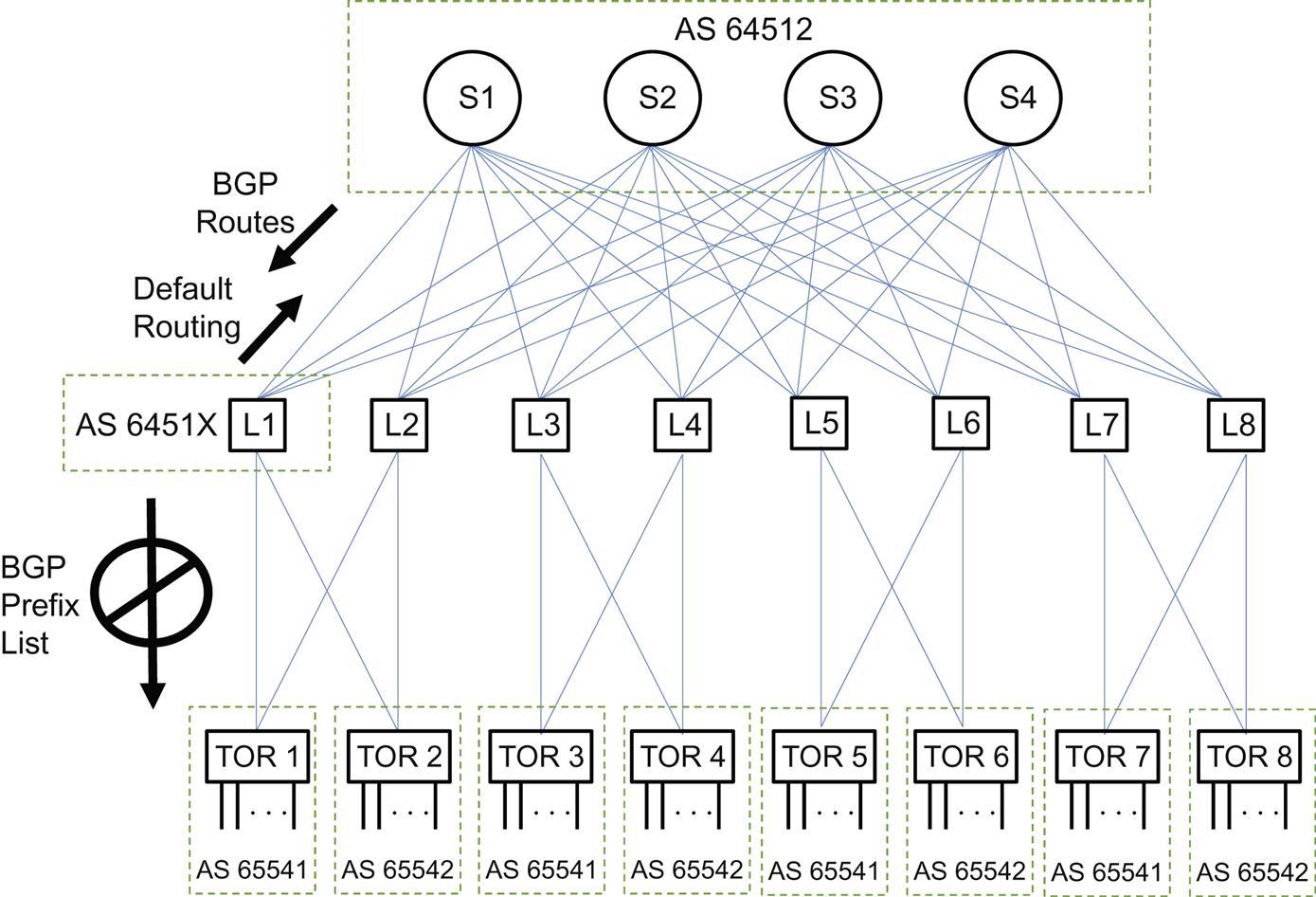
What we’ve done so far is shown in Figure 17.9. And this system works fine—up to a point.

Now, in truly huge (“large-scale”) data center, we quickly run out of suitable private AS numbers. We could always use 32-bit private ASNs, but these are unfamiliar and located in an odd range. But we could also reuse ASNs for each quad cluster. This reuse requires that the spine AS devices enable the BGP “Allow AS In” option, but that is seldom an issue for modern BGP implementations.
What IP addresses should these eBGP sessions distribute in its NLRIs? If we advertise all the link addresses, then there is little advantage over using an IGP as the data center scales to thousands of servers. It’s also not clear why the spine switches would need to know the addresses of a link between L1 and TOR2 and what the next hop might be. But eBGP can use the loopback address of each individual router (the switches must also employ Layer 3 if they are running BGP) for that purpose. Server subnets still need to be known and announced by BGP, but reaching the servers is the main goal. Also, because of the way that CLOS networks function, summarization of IP addresses would lead to black-holing traffic (any further discussion of this point is beyond the bounds of this summary chapter).
To connect through a gateway router beyond the Clos structure, to a WAN or the Internet or another data center, this data center needs to conceal the private ASNs used. However, this is necessary even for a single private AS when used for an enterprise network. And from leaf to spine, we can rely on a default route to direct traffic up to the spine and beyond the data center for external reachability.
Note that we still inject BGP routes from the spine and gateways to the leafs because external destination must still be known. But for “outbound” traffic, only a default route (“if you don’t know where to send it, send it here”) is needed. Finally, notice that we do not distribute the full BGP prefix list on the quads from the leafs to the TOR switches.
BGP can use ECMP to distribute traffic headed for the same IP address across multiple links if they have the same underlying metrics. Usually, this just means that all links in the data center run at the same speed.
However, when a leaf device loses a path for a prefix, it still has a default route to the spine device. For a period of time, usually short, the spine device might still have a path that leads to the leaf device. This creates a short-lived “micro-loop” in the network. To avoid this, we can configure “discard routes” on the leafs switches to make sure that traffic heading for the TOR switch does not bounce back to the spine devices because of the default route.
One example use of eBGP in the data center is shown in Figure 17.9. In our modest network, there really is very little gain over using an IGP to establish reachability. In fact, iBGP could be used with a route reflector (RR: there are virtual route reflectors specialized for use in the data center) to cut down on peering requirements. But standard RR devices only reflect the “best” prefix and so struggle with ECMP unless the device supports the BGP “AddPath” feature. Optimized Route Reflection (ORR), discussed earlier in this chapter, can address this issue (Figure 17.10).
In any case, as the data center scales into the “hundreds of thousands of servers” range (as the draft explicitly mentions), BGP becomes more and more attractive for use in the data center network.
Distributing Link-State Information with BGP
As we have seen, routers and other type of network nodes use an IGP to distribute routing information inside a routing domain or AS. IGP determines which routes are the best candidates to distribute using one of two methods:
• Distance vector—This technique is used by older protocols such as the routing information protocol (RIP). These protocols advertise the entire routing table to their directly connected neighbors using a broadcast address (“Everybody, pay attention to this!”). The best path to a destination is simply the minimum number of hops (routers or network nodes) that the packet would take to the destination, regardless of link speed or node processing power.
• Link-state protocols—This technique, used by protocols such as OSPF or IS-IS, advertise information about the network topology to all routers in a routing domain using multicast addresses (“If you are interested, pay attention to this”). This triggers other updates until all routers running the protocol have the same information about the network, a process known as convergence. Best paths can then be determined by different criteria: delay, bandwidth, or other parameters.
Whatever the method, the IGP provides routing connectivity information within the routing domain, the set of routers under common control of a single administration entity that controls the domain. A BGP AS can contain a single routing domain (the simplest case) or several, and these separate domains can even run different IGPs. Inside an AS, the IGP(s) learns reachable prefixes and the interfaces to reach them and advertised the “best” way to get to them to all IGP neighbors. When an AS consists of multiple routing domains, the IGPs can exchange information gathered from different routing protocols through a process known as route redistribution. This redistribution ties multiple routing domains together inside a single AS (so the routes are still intra-AS and not external routes).
The IGP Limitations
No matter which IGP is used inside a routing domain, IGPs are limited when scaling and in performance (link-state calculation and convergence time). IGPs have to take into account all types of traffic engineering considerations to determine the link state (we don’t usually think of link bandwidth as an aspect of traffic engineering, but static parameters count as much as dynamic ones like queue length).
IGPs struggle with large databases and have the added limitation of viewing only as portion of the entire global network, limiting their ability to calculate end-to-end traffic engineering results. Once a path from source to destination breaks out of the sphere of the IGP routing domain, traffic engineering considerations break down because complete routing information is not available to all routers.
What we would like to have is a way to get IGP link-state information from one routing domain to another, whether the routing domains are inside one AS or not. If the routing domains are different ASs and have different ISPs, the ISP can agree to share their link-state information without enabling global distribution and the resulting confidentiality and scaling issues.
Fortunately, we can use a form of spanning link-state distribution with BGP.
The BGP Solution
As soon as IGP information is needed outside a routing domain, an EGP is needed. The EGP can get link-state, traffic engineering, and other information from an IGP and share it across the routing boundary to enable computation of effective inter-domain paths.
Naturally, BGP is the standard EGP used for this purpose. If BGP can carry information about every prefix on the global public Internet everywhere, it can be extended to handle this aspect of routing as well. In contrast to IGPs, BGP does not use broadcast or multicast addressing to send out information, but uses TCP session to designated peers (“You, and you alone, pay attention to this”). This cuts down on the amount a time a server or other device (anything not a router) on the same LAN as a router spends parsing frames and packets that contain nothing of interest to the destination (except for potential hackers, or course). The use of TCP enables peers to employ flow control during periods of routing information “churn” be delaying TCP acknowledgments, something that IGPs are unable to do.
As we have seen before, the extensible nature of BGP NLRIs provide a nice platform for adding capabilities without compatibility concerns or altering the basic protocol. Also, BGP routing polices provide excellent control over exactly what information is sent to peers and what information each peer will accept. The BGP routing policies can also filter and modify the information inside the NLRIs.
Inside an AS, however, IGP and BGP are distributing the same set of traffic engineering parameters (hopefully, BGP polices are not altering bandwidth and other characteristics within a routing domain). But BGP scales more gracefully than the IGP. The information acquired by the IGP can be aggregated by BGP and distributed even beyond the AS is desired (and allowed). In these days of control plane separation, BGP can be used by a central or external path computation entity to passively listen to a route reflector for all the traffic engineering and link-state information it needs.
In summary, if we want a way to distribute IGP link-state information beyond the reach of the IGP, then BGP is that way to do it.
Implementing BGP for Link-State Protocols
How should routers implement this new capability for BGP? The standards say that there should be a “protocol agnostic representation” of nodes and links for these purposes. This is a fancy way of saying that any implantation should be more abstract than the concrete link-state parameters used by the IGP for nodes and links.
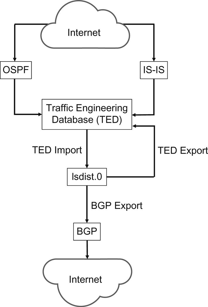
Because the Illustrated Network is built out of Juniper Networks equipment, let’s look in a bit more detail at how Juniper Networks routers implement sharing link-state information across IGP boundaries using BGP. The “protocol agnostic” database for this information already exists in every Juniper Networks router (and other Layer 3 devices) as the Traffic Engineering Database (TED). All topology information is also in the TED. All that is missing is a way to “transcode” this link-state information into a format suitable for BGP NLRI updates.
To do this, we’ll put all relevant link-state information into a separate table called the “link-state distribution table,” or lsdist.0. All of the link and nodes entries in the TED are converted into routes before being placed into the TED table, a process called TED import, and users can examine these entries if they wish. In fact, a routing policy can be inserted here to control exactly which routes are “leaked” into the lsdist.0 table. Then we can export this collected information back into the TED (because it is a cumulative process) and out to BGP for export to peers. This overall process is shown in Figure 17.11.
Another policy can be used to export (advertise) routes from the lsdist.0 table using BGP. To do this, BGP needs to be configured with the BGP-TE address family and an export policy to select these routes for BGP distribution.
BGP then sends these routes as it would any other NLRIs. BGP peers that have the BGP-TE address family enabled receive and process these BGP-TE NLRIs, storing them in the receiver’s lsdist.0 table.
All routes in the lsdist.0 table must be selected for export with a routing policy. By default, no entries are leaked from the lsdist.0 table unless directed by a policy.
One other aspect of Juniper Network’s link-state BGP distribution should be mentioned. That is the fact that the TED uses a protocol preference scheme based on the protocol used to provide the information to the table. Entries learned by BGP can be supplied by different protocols, and TED entries can correspond to more than one protocol. To make sense out of this multiplicity, a protocol with a higher “credibility” value is favored over a source with a lower value. The credibility values can be changed by configuration.
Juniper Network’s Implementation Details
The Junos OS implements distribution on BGP-TE NLRIs through route reflector. The following list of NLRIs are supported:
Juniper Networks does not support the route-distinguisher form of these NLRI.
With respect to the node and link NLRI’s the Junos OS supports the following fields:
• Protocol-ID—NLRI origins with the following protocol values:
• Identifier—This value is configurable. By default, the identifier value is set to 0
• Local/Remote node descriptor, which include:
• BGP-LS Identifier—This value is configurable. By default, the BGP-LS identifier value is set to 0
• Link descriptors (only for the link NLRI), which include:
• Link Local/Remote Identifiers
• IPv6 neighbor/interface address—The IPv6 neighbor and interface addresses are not originated, but only stored and propagated when received
• Multi-topology ID—This value is not originated, but stored and propagated when received.
The following is a list of supported LINK_STATE attribute TLVs:
• Maximum reservable bandwidth
• The following TLVs, which are not originated, but only stored and propagated when received:
• Node flag bits—Only the overload bit is set
• The following TLVs, which are not originated, but only stored and propagated when received:
• OSPF-specific node properties
• Prefix attributes—These TLVs are stored and propagated like any other unknown TLVs.
Summary of Supported and Unsupported Features
The Junos OS supports the following features with link-state distribution using BGP:
• Advertisement of multiprotocol assured forwarding capability
• Transmission and reception of node and link-state BGP and BGP-TE NLRIs
The Junos OS does not support the following functionality for link-state distribution using BGP:
• Aggregated topologies, links, or nodes
• Route distinguisher support for BGP-TE NLRIs
• Multi-instance identifiers (excluding the default instance ID 0)
• Advertisement of the link and node area TLV
• Advertisement of MPLS signaling protocols
• Importing node and link information with overlapping address.
Configuring BGP-LS on the Illustrated Network
In the previous chapter, we’ve already split the Illustrated Network into two AS routing domains and put core routers P9 and P4 in one AS (AS 65531) along with edge router PE5, and P7 and P2 in another (AS 65527). We configured iBGP on router P9 to make router P4 and PE5 iBGP internal neighbors and eBGP to make routers P7 and P2 external neighbors of P9.
Here’s all we had to do on router P9 to establish eBGP sessions to routers P7 and P2.
set protocols bgp group ebgp ebgp-to-as65527 type external;
set protocols bgp group ebgp ebgp-to-as65527 peer-as 65527;
set protocols bgp group ebgp ebgp-to-as65527 neighbor 10.0.79.1;
set protocols bgp group ebgp ebgp-to-as65527 neighbor 10.0.29.1;
We also had an iBGP group to peer with routers P4 and PE5.
set protocols bgp group ibgp-mesh type internal;
set protocols bgp group ibgp-mesh local-address 192.168.9.1;
set protocols bgp group ibgp-mesh neighbor 192.168.4.1;
set protocols bgp group ibgp-mesh neighbor 192.168.5.1;
(Note the peering to router loopback addresses for internal peers and interface addresses for eBGP.)
Now let’s add the statements needed on a Juniper Networks router to create the lsdist.0 TED table on router P9 using the metrics received from an IGP (in this case, we’ll use OSPF).
The first thing we have to do on router P9 is to allow OSPF to use traffic engineering link-state advertisements (LSAs) in the first place on the links to P4 and PE5 that run the IGP.
set protocols ospf traffic-engineering
set protocols ospf area 0.0.0.0 interface s0-0/0/0 traffic-engineering remote-node-id 10.0.59.1
set protocols ospf area 0.0.0.0 interface s0-0/0/0 traffic-engineering remote-node-router-id 192.168.5.1
set protocols ospf area 0.0.0.0 interface s0-0/0/3 traffic-engineering remote-node-id 10.0.49.1
set protocols ospf area 0.0.0.0 interface s0-0/0/3 traffic-engineering remote-node-router-id 192.168.4.1
For reasons that are far beyond the scope of this introductory chapter, it’s also a good practice to run OSPF in passive mode (i.e., without worrying about a full exchange of routing information) on the interfaces they are also running eBGP, i.e., P7 and P2 in AS 65527.
set protocols ospf area 0.0.0.0 interface s0-0/0/1 passive traffic- engineering remote-node-id 10.0.79.1
set protocols ospf area 0.0.0.0 interface s0-0/0/1 passive traffic- engineering remote-node-router-id 192.168.7.1
set protocols ospf area 0.0.0.0 interface s0-0/0/2 passive traffic- engineering remote-node-id 10.0.29.1
set protocols ospf area 0.0.0.0 interface s0-0/0/2 passive traffic- engineering remote-node-router-id 192.168.2.1
Now we can also configure eBGP with the only other statement needed to use traffic engineering LSAs and NLRIs.
set protocols bgp group ebgp ebgp-to-as65527 type external;
set protocols bgp group ebgp ebgp-to-as65527 family traffic-engineering unicast;
set protocols bgp group ebgp ebgp-to-as65527 peer-as 65527;
set protocols bgp group ebgp ebgp-to-as65527 neighbor 10.0.79.1;
set protocols bgp group ebgp ebgp-to-as65527 neighbor 10.0.29.1;
In order to get traffic engineering information from AS65527, we would add traffic engineering to our iBGP peers as well.
set protocols bgp group ibgp-mesh type internal;
set protocols bgp group ibgp-mesh family traffic-engineering unicast;
set protocols bgp group ibgp-mesh local-address 192.168.9.1;
set protocols bgp group ibgp-mesh neighbor 192.168.4.1;
set protocols bgp group ibgp-mesh neighbor 192.168.5.1;
What about the routing policies needed to get link-state information into and out of the TED table? Those are not difficult to configure either.
set policy-options policy-statement bgp-to-ted from family traffic-engineering;
set policy-options policy-statement bgp-to-ted then accept;
When applied, this policy takes all BGP NRLI updates concerning traffic engineering (i.e., our link-state information from the IGP) and places it into the TED. To export this information to other routers is a simple policy as well (and also uses next-hop self):
set policy-options policy-statement nlri-bgp term 1 from family traffic- engineering;
set policy-options policy-statement nlri-bgp term 1 then next-hop self;
set policy-options policy-statement nlri-bgp term 1 then accept;
Normally, we would apply these polices to interface or protocols, but we haven’t discussed one of the most common protocol families used with traffic engineering. This family is Multiprotocol Label Switching (MPLS), but we will have to wait for a couple of chapters to talk about statements like these:
set protocols mpls traffic-engineering database import policy ted-to-nlri;
set protocols mpls cross-credibility-cspf
Let’s close by saying that the cross-credibility statement allows the router to create constrained shortest path first (CSPF) ways through the network using traffic engineering information from more than one source, such as OSPF and IS-IS.
Questions for Readers
1. What is ORR and what does it do?
2. What does a RTBH do and what are two ways that these mechanisms can be triggered?
3. What is a CLOS network and what form of CLOS network is often used in a large data center?
4. Why consider BGP for use in a large data center? Discuss at least four reasons.
5. Compare very large data center use of IGP with use of eBGP.