TensorFlow is an open source software library that focuses on high-performance numerical computation and deep learning with access and support to CPUs, GPUs, and TPUs (Tensor Process Units, new Google hardware specialized for deep learning purposes). This library is not an easy library and has a high learning curve, but the introduction of Keras (a library on top of TensorFlow) as a part of TensorFlow makes the learning curve easier, but still requires a huge learning curve itself.
In this chapter, we cannot explain how to use TensorFlow because we will require a separate book for this topic alone, but we are going to explain the structure of the CNN we are going to use. We will show how to use an online visual tool called TensorEditor to generate, in a few minutes, TensorFlow code that we can download and train locally on our computer, or use the same online tool to train our model if we don't have enough computer processing power. If you want to read about and learn TensorFlow, we suggest you read any of the relevant Packt Publishing books or the TensorFlow tutorials.
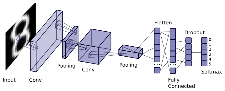
The CNN layer structure that we are going to create is a simple convolutional network:
- Convolutional Layer 1: 32 filters of 5 x 5 with ReLU activation function
- Pooling Layer 2: Max pooling with 2 x 2 filters and a stride of 2
- Convolutional Layer 3: 64 filters of 5 x 5 with ReLU activation function
- Pooling Layer 4: Max pooling with 2 x 2 filter and a stride of 2
- Dense Layer 5: 1,024 neurons
- Dropout Layer 6: Dropout regularization with a rate of 0.4
- Dense Layer 7: 30 neurons, one for each number and character
- SoftMax Layer 8: Softmax layer loss function with gradient descent optimizer with a learning rate of 0.001 and 20,000 training steps.
We can see a basic graph of the model we have to generate in the following diagram:
TensorEditor is an online tool that allows us to create models for TensorFlow and train on the cloud, or download the Python 2.7 code and execute it locally. After registering for the online free tool, we can generate the model, as shown in the following diagram:
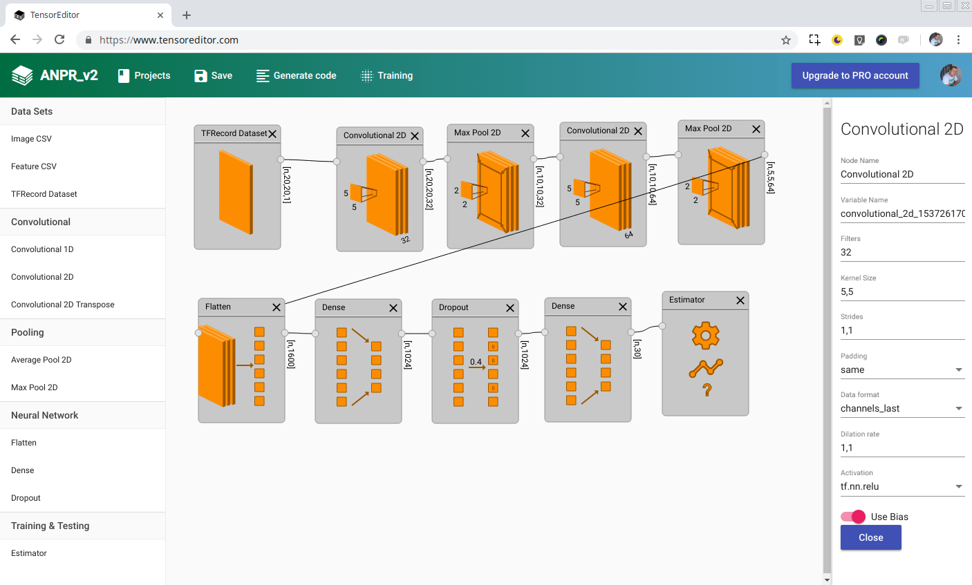
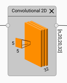
To add a layer, we choose it by clicking on the left-hand menu and it will appear on the editor. We can drag and drop to change its position and double-click to change its parameters. Clicking on the small dots of each node, allows us to link each node/layer. This editor shows us the parameters we choose visually and the output size of each layer; we can see in the following image that the convolutional layer has a kernel of 5 x 5 x 32 and an output of n x 20 x 20 x 32; the n variable means that we can compute one or multiple images at the same time for each training epoch:
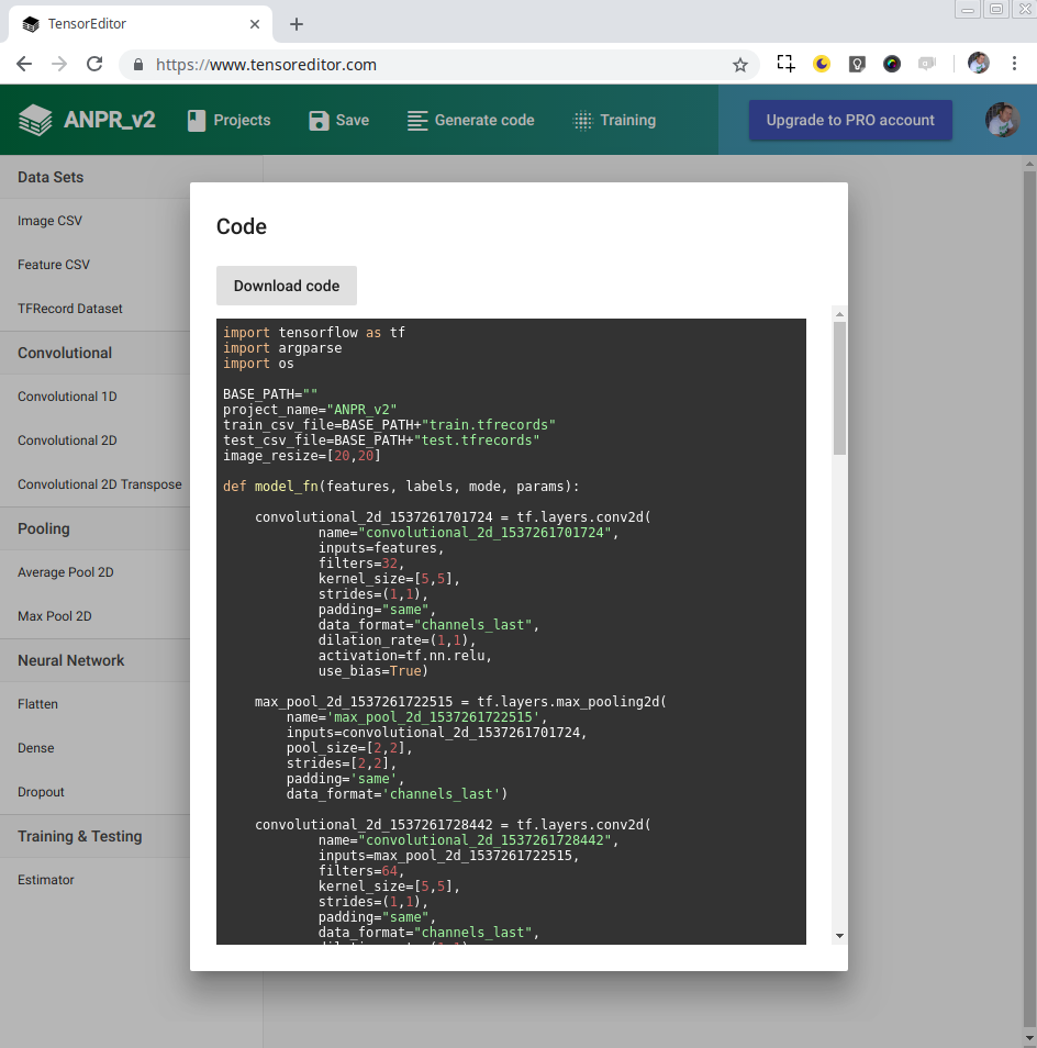
After creating the CNN layer structure in TensorEditor, we can now download the TensorFlow code by clicking on Generate code and downloading the Python code, as shown in the following screenshot:
Now, we can start training our algorithm using TensorFlow with the following command:
python code.py --job-dir=./model_output
Here, the --job-dir parameter defines the output folder in which we store the output model trained. In the terminal, we can see the output of each iteration, together with the loss result and accuracy. We can see an example in the following screenshot:

We can use TensorBoard, a TensorFlow tool, which gives us information about the training and graphs. To activate TensorBoard, we have to use this command:
tensorboard --logdir ./model_output
Here, the --logdir parameter, where we save our model and checkpoints, must be identified. After launching TensorBoard, we can access it with this URL: http://localhost:6006. This awesome tool shows us the graph generated by TensorFlow, where we can explore every operation and variable, clicking on each node, as we can see in the next screenshot:

Or, we can explore the results obtained, such as for loss values in each epoch step or accuracy metrics. The results obtained with the training model per epoch are shown in the following screenshot:
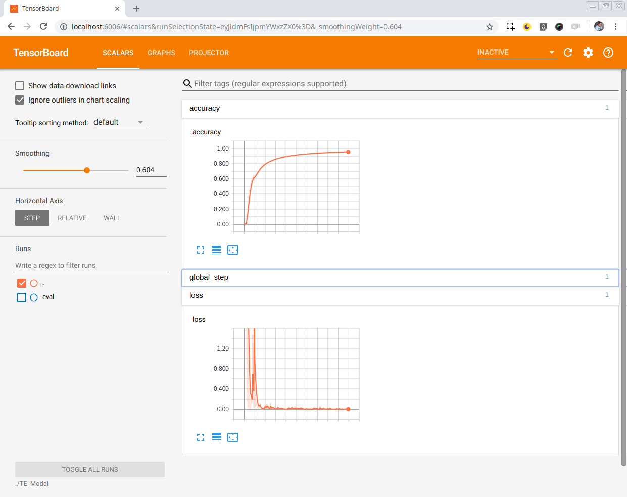
Training on an i7 6700HQ CPU with 8 GB RAM takes a long time, around 50 hours; a bit more than two days of training. If you use a basic NVIDIA GPU, this task can be reduced to around 2-3 hours.
If you want to train in TensorEditor, it can take 10-15 minutes and will download the model after training the models, with the possibility of downloading the full output model or a frozen and optimized model. The concept of freezing will be described in the following section, Preparing a model for OpenCV. We can see the result of training in TensorEditor in the next screenshot:

Analyzing the results obtained, we attain an accuracy level of around 96%, much better than the old algorithm explained in the second edition of this book, where we attained an accuracy level of only 92% using feature extraction and a simple artificial neural network.
After we finish training, all models and variables are stored in the job folder defined when we launched the TensorFlow script. Now, we have to prepare the finished result to integrate and import it into OpenCV.