Chapter 4

Traveling About the Stack

IN THIS CHAPTER

Moving about the stack

How local variables are stored

Viewing threads and memory

Tracing through assembly code

Debuggers can be powerful things. They can leap tall computer applications in a single bound and see through them to find all their flaws. The more you know about debuggers, the more you can put them to use. In this chapter, you see how to move about the stack, which provides you with a record of calls within your application, among other useful information.

This chapter also helps you view data in various ways. For example, in the previous chapter you got a quick view of local variables in the “Watching the variables” section. This chapter enhances your understanding of local variables. In addition, you see how threads and memory work, which offers another perspective of data and how code interacts with it. Finally, you get down to the nuts and bolts with assembly language, which is sort of the way that the computer sees your application, except with a human-readable twist.

You don’t have to type the source code for this chapter manually. In fact, using the downloadable source is a lot easier. You can find the source for this chapter in the \CPP_AIO4\BookIV\Chapter04 folder of the downloadable source. See the Introduction for details on how to find these source files.

Stacking Your Data

A stack is a common data structure in the computer world. When the operating system runs an application, it gives that application a stack, which is simply a big chunk of memory used to store data. But the data is stored just like a stack of cards (or a stack of pancakes if you prefer): With a stack of real cards, you can put a card on the top, and then another, and do that six times over; then you can take a card off and take another card off. You can put cards on the top and take them off the top. And if you follow these rules, you can’t insert them into the middle or bottom of the stack. You can only look at what’s on the top. A stack data structure works the same way: You can store data in it by pushing the data onto the stack, and you can take data off by popping it off the stack. And yes, because the stack is just a bunch of computer memory, sneaking around and accessing memory in the middle of the stack is possible. But under normal circumstances, you don’t do that: You put data on and take data off.

What’s interesting about the stack is that it works closely with the main CPU in your system. The CPU has its own little storage bin right on the chip itself. (It isn’t in the system memory, or RAM; it’s inside the CPU itself.) This storage bin holds what are called registers. One such register is the stack pointer, called the SP when working with 16-bits, ESP when working with 32-bits, or RSP when working with 64-bits. The names of the registers vary by register size. When the folks at Intel replaced the earlier chips with newer, more powerful chips, they made the registers bigger. You can see a listing of register names at https://docs.microsoft.com/en-us/windows-hardware/drivers/debugger/x64-architecture. The tutorial at https://www.tutorialspoint.com/assembly_programming/assembly_registers.htm provides additional information as well.@@@

The stack is useful in many situations and is used extensively behind the scenes in the applications you write. The compiler generates code that uses the stack to store:

• Local variables
• Function parameters
• Function calling order

It’s all stacked onto the stack and stuck in place, ready to be unstacked.

Moving about the stack

The Code::Blocks debugger, like most debuggers, lets you look at the stack. But really, you’re not looking directly at the hardware stack. When a debugger shows you the application stack, it’s showing you the list of function calls that led up to the application’s current position in the application code. However, the application stack is a human-readable form of the hardware stack, and the debugger uses the hardware stack to get that information. So that’s why programmers always call the list of function calls the stack, even though you’re not actually looking at the hardware stack.

Figure 4-1 shows an example of the Call Stack window in Code::Blocks. To see the Call Stack window, simply choose Debug⇒  Debugging Windows⇒  Call Stack. You can see the Call Stack window in front of the main Code::Blocks window. No information appears in the Call Stack window until you start running an application.

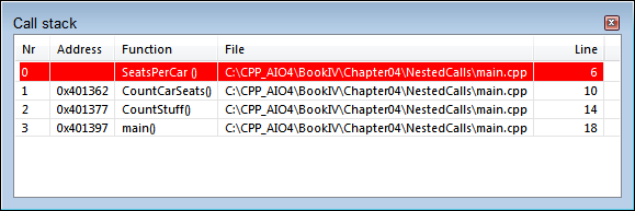
FIGURE 4-1: The Call Stack window shows the function calls that led up to the current position.

You can try viewing the stack yourself. Look at the NestedCalls example, shown in Listing 4-1. This listing shows a simple application that makes several nested function calls.

LISTING 4-1: Making Nested Function Calls

#include <iostream>

using namespace std;

int SeatsPerCar() {
return 4;
}

int CountCarSeats() {
return 10 * SeatsPerCar();
}

int CountStuff() {
return CountCarSeats() + 25;
}

int main() {
cout << CountStuff() << endl;
// Remove the following comment to see the code
// execute in the debugger.
//system("PAUSE");
return 0;
}

To try the Call Stack window, follow these steps:

1. Compile this application (set the Build Target field to Debug).
2. Set a breakpoint at the cout << CountStuff() << endl; line.
3. Run the application in the Code::Blocks debugger by pressing F8.

4. Step into the CountStuff() function, and then into the CountCarSeatsfunction(), and then into the SeatsPerCar() function.

   (Or, just put a breakpoint in the SeatsPerCar() function and run the application until it stops at the breakpoint.)

5. Choose Debug⇒  Debugging Windows⇒  Call Stack.

   A window like the one in Figure 4-1 appears. Note the order of function calls in the Call Stack window:

   SeatsPerCall()
CountCarSeats()
CountStuff()
main()

   This information in the Call Stack window means that your application started with main(), which called CountStuff(). That function then called CountCarSeats(), which in turn called SeatsPerCall(). And that’s where you are now. Code::Blocks places a red highlight on the current stack location — the block of code that the application is currently executing.

This window is handy if you want to know what path the application took to get to a particular routine. For example, you might see a routine that is called from many places in your application and you’re not sure which part is calling the routine when you perform a certain task. To find out which part calls the routine, set a breakpoint in the function. When you run the application and the debugger stops at that line, the Call Stack window shows you the path the computer took to get there, including the name of the function that called the function in question.

In the Call Stack window, you can double-click any function name, and the Debugger moves the cursor to the function’s body in the source code. This feature makes it easy for you to locate any function within the call stack and see why the code followed the path it did. Double-clicking only moves your view to the line on the call stack; the program is still stopped on the line at the top of the stack. When you switch to a new location in the call stack, the red bar moves to that location in the Call Stack window so that you can always keep track of where you are in the call stack.

Stack features are common to almost all debuggers. It’s not possible to say all, because some truly bad debuggers that don’t have stack features are out there. But the good debuggers, including those built into Code::Blocks and Microsoft Visual C++, include features for moving about the stack.

Storing local variables

As you get heavily into debugging, it always helps to fully understand what goes on under the hood of your application. At this point, the text speaks on two levels:

• Your C++ code
• The resulting assembly code that the compiler generates based on your C++ code. (Assembly is the human-readable form of machine code that the processor on your machine understands.)

This chapter clearly states which level you’re reading about. Suppose that you write a function in C++ and you call the function in another part of your application. When the compiler generates the assembly code for the function, it inserts some special code at the beginning and end of the function. At the start of the function, this special code allocates space for the local variables. At the end of the function, the special code de-allocates the space. This space for the variables is called the stack frame for the function.

This space for the local variables lives on the stack. The storage process works as follows: When you call your function, the computer pushes the return address of the caller onto the stack. After the computer is running inside the function, the special code that the compiler inserted saves some more of the stack space — just enough for the variables. This extra space becomes the local storage for the variables, and just before the function returns, the special code removes this local space. Thus, the top of the stack is now the return address. The return then functions correctly.

This process with the stack frame takes place with the help of the internal registers in the CPU. Before a function call, the assembly code pushes the arguments to the function onto the stack. Then it calls the function by using the CPU’s built-in call statement. (That’s an assembly-code statement.) This call statement pushes the return address onto the stack and then moves the instruction pointer to the function address. After the execution is inside the function, the stack contains the function arguments and then the return address. The special function start-up code (called a prolog) saves the beginning of the stack frame address in one of the CPU registers, called the Base Pointer (BP) register. (As with SP, the name of BP can be EBP or RBP based on the register size.)

The prolog saves the value on the stack. The prolog code first pushes the BP value onto the stack. Then the prolog code takes the current stack pointer (which points to the top of the stack in memory) and saves it back in the BP register for later use. Then the prolog code adjusts the stack pointer to make room for the local variable storage. The code inside the function then accesses the local variables as offsets above the position of BP on the stack and the arguments as offsets below the position of BP on the stack.

Finally, at the end of the function, the special code (now called an epilog) undoes the work: The epilog copies the value in BP back into SP; this de-allocates the local variable storage. Then it pops the top of the stack off and restores this value back into BP. Now the top of the stack contains the function return address, which is back to the way it was when the function began. The next assembly statement is a return, which pops the top of the stack off and goes back to the address that the epilog code popped off the stack. Just think: Every single time a function call takes place in your computer, this process takes place.

Inside the computer, the stack actually runs upside down. When you push something onto the stack, the stack pointer goes down in memory — it gets decremented. When you pop something off the stack, the stack pointer gets incremented. Therefore, in the stack frame, the local variables are actually below BP in memory, and you access their addresses by subtracting from the value stored in the BP register. The function arguments, in turn, are above the BP in memory, and you get their addresses by adding to the value stored in BP.

The one topic not discussed in the preceding paragraph is the return value of a function. In C++, the standard way to return a value from a function is for the function’s assembly code to move the value into the Accumulator, or AX, register (whose name also varies by register size). The calling code can inspect the AX register after the function is finished. However, if you are returning something complex, such as a class instance, things get a bit more complex. Suppose that you have a function that returns an object, but not as a pointer, as in the function header MyClass MyFunction();. Different compilers handle this differently, but when the gcc compiler that’s a part of Code::Blocks, Dev-C++, MinGW, or Cygwin encounters something such as MyClass inst = MyFunction();, it takes the address of inst and puts it in AX. Then, in the function, it allocates space for a local variable, and in the return line it copies the object in the local variable into the object whose address is in AX. So when you return a non-pointer object, you are, in a sense, passing your object into the function as a pointer.

Debugging with Advanced Features

Most debuggers, including Code::Blocks, have some advanced features that are handy when you’re tracing through your application. These features include the capability to look at threads (individual sequences of programmed instructions) and assembly code.

Viewing threads

If you are writing an application that uses multiple threads and you stop at a breakpoint, you can get a list of all current threads by using the Running Threads window. To open the Running Threads window, in the main Code::Blocks window choose Debug⇒  Debugging Windows⇒  Running Threads. A window showing the currently running threads opens. Each line looks something like this:

2 thread 2340.0x6cc test() at main.cpp:7

The first number indicates which thread this is in the application; for example, this is the second thread. The two numbers after the word thread are the process ID and the thread ID in hexadecimal, separated by a dot. Then you see the name of the function where the thread is stopped, along with the line number where the thread is stopped.

Tracing through assembly code

If you feel the urge, you can view the actual assembly code. In some cases, you use the assembly code view to find particularly difficult bugs, or you might want to determine which of two programming techniques produces less code. In fact, you may just be curious as to how the compiler converts your code. To see the assembly code, choose Debug⇒  Debugging Windows⇒  Disassembly and you see the Disassembly window. Check the Mixed Mode option when you want see a mix of C++ and assembly code, as shown in Figure 4-2. This approach makes it a lot easier to understand how Code::Blocks turns your C++ code into assembly language. Notice that the top of the window tells you the name of the function you’re viewing and which file contains the function, and the C++ code includes line numbers so that you know precisely where you are in the source code.

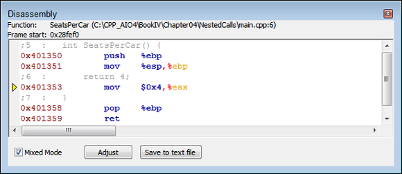
FIGURE 4-2: The Disassembly window shows the assembly code that results from the C++ code you write.

Some readers have noted that Code::Blocks will sometimes freeze when displaying the Disassembly window. The IDE will report that the disassembly is being loaded, but the process never completes. In this case, close the sample code and restart the IDE. In most cases, the disassembly will load on the second try.

The window shown in Figure 4-2 is the disassembly of the SeatsPerCar() function shown previously in Listing 4-1. Here’s the function again so that you can compare it to Figure 4-2:

int SeatsPerCar() {
return 4;
}

The following lines create the stack frame:

0x401350 push %ebp
0x401351 mov %esp,%ebp

You know that this is a 32-bit application because the disassembly uses the 32-bit register names throughout. If this were a 64-bit application, the register names would reflect the proper size, such as %rbp and %rsp.

After the code creates a stack frame, it moves a value of 4 (the return 4; part of the code) into EAX, as shown here:

0x401353 mov $0x4,%eax

The code then pops EBP and returns to the caller (the CountCarSeats() function) using this code:

0x401358 pop %ebp
0x401359 ret

Now, if you move into the CountCarSeats() function, you see assembly like that shown in Figure 4-3.

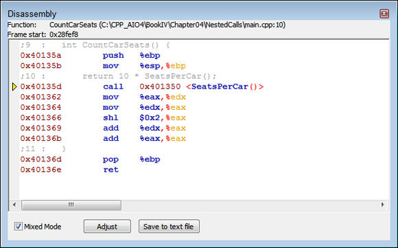
FIGURE 4-3: This Disassembly window shows the CountCarSeats() function code.

As before, the assembly code begins by creating a stack frame. It then issues a call to the SeatsPerCar() function. When the function returns, the assembly performs the multiplication part of the task. Finally, the code performs the usual task of placing the return value in EAX, popping EBP, and returning to the caller. Notice that what appears to be simple multiplication to you may not be as simple in assembly language. Say that you change the code to read

int CountCarSeats() {
return 4 * SeatsPerCar();
}

The math is simpler now because you’re using 4, which is easily converted into a binary value. Figure 4-4 shows the assembly that results from this simple change.

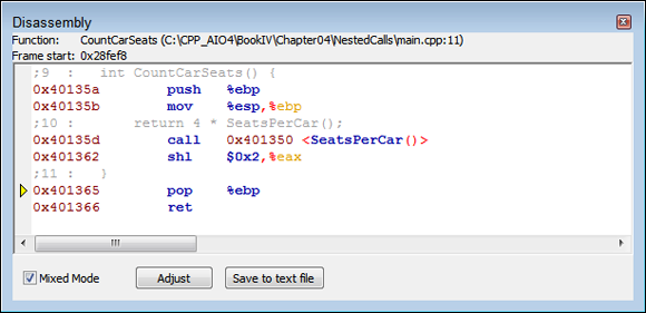
FIGURE 4-4: Small C++ code changes can result in large assembly-code changes.

Now all the code does is perform a shift-left (SHL) instruction. Shifting the value in EAX left by 2 is the same as multiplying it by 4. The assembler uses the SHL instruction because shifting takes far fewer clock cycles than multiplication, which makes the code run faster. The result is the same, even if the assembly code doesn’t quite match your C++ code.

If you want to see the values in the registers so that you can more easily follow the assembly code, choose Debug⇒  Debugging Windows⇒  CPU Registers. You see the CPU Registers window, shown in Figure 4-5. This window reflects the state of the registers at the current stopping point in the code. Consequently, you can’t see each step of the assembly code shown in the Disassembly window reflected in these registers unless you step through the code, one instruction at a time.

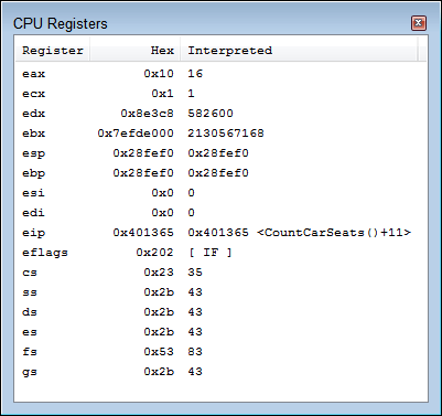
FIGURE 4-5: Viewing the CPU registers can give you insight into how code interacts with the processor.