IFS Function

The IFS function enables you to carry out multiple logical tests and execute a statement that corresponds to the first test that is TRUE. The tests need to be entered in the order in which you want the statements executed so that the right result is returned as soon as a test is passed. IFS can be used in place of nested IF statements which can quickly become too complex.

For example, the statement below has 4 nested IF functions:

=IF(D2>69,"A",IF(D2>59,"B",IF(D2>49,"C",IF(D2>39,"D","F"))))

The formula can be made much simpler with a single IFS function:

=IFS(D2>69,"A",D2>59,"B",D2>49,"C",D2>39,"D",TRUE,"F")

As you can see with the IFS variant, you don’t need to worry about all the IF statements and parentheses.

Syntax

IFS(logical_test1, value_if_true1, [logical_test2, value_if_true2], [logical_test3, value_if_true3],…)

Arguments

Argument	Description
logical_test1	Required. This is the condition that is being tested. It can evaluate to TRUE or FALSE.
value_if_true1	Required. The result to be returned if logical_test1 evaluates to TRUE.
logical_test2… logical_test127	Optional. You can add up to 127 additional tests that evaluate to TRUE or FALSE.
value_if_true2… value_if_true127	Optional. You can have up to 127 additional results to return if a logical test is true.

Note : The IFS function allows you to test up to 127 different tests. However, it is generally recommended that you do not use too many tests with IF or IFS statements. This is because the tests need to be entered in the right order and it can become too complex to update or maintain if you have too many.

Tip : As much as possible, use IFS in place of multiple nested IF statements. It is much easier to read when you have multiple conditions.

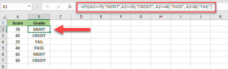
Example 1

In the example below, we use the IFS function to solve a problem we addressed earlier with nested IF statements.

In this problem, we want to assign grades to different ranges of exam scores.

Score and Grades

1. 70 or above = MERIT
2. 50 to 69 = CREDIT
3. 40 to 49 = PASS
4. less than 40 = FAIL

We derive the following formula to achieve our aim:

=IFS(A2>=70,"MERIT",A2>=50,"CREDIT", A2>=40,"PASS", A2<40,"FAIL")

Formula explanation

=IFS(A2>=70,"MERIT",A2>=50,"CREDIT", A2>=40,"PASS", A2<40,"FAIL")

The IFS function as been used to create four logical tests in sequential order:

A2>=70,"MERIT"

A2>=50,"CREDIT"

A2>=40,"PASS"

A2<40,"FAIL"

A2 is a reference to the score. As you can see, each score is tested against each condition in sequential order. As soon as a test is passed the corresponding grade is returned and no further testing is carried out.

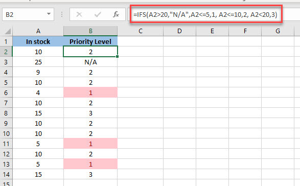
Example 2

In this example, we want to set different priority levels for reordering items depending on the number of items in stock.

Priority Level:

1. 5 or less = 1
2. 10 or less = 2
3. Less than 20 = 3

The formula we use to accomplish this task is:

=IFS(A2>20,"N/A",A2<=5,1, A2<=10,2, A2<20,3)

Formula explanation

=IFS(A2>20,"N/A",A2<=5,1, A2<=10,2, A2<20,3)

First, we insert a test to mark the Priority Level for any products greater than 20 as “N/A” (not applicable) as those have no Reorder priority yet. Then we carry out the tests in sequential order from the smallest value to the largest to ensure that the right corresponding value is returned as soon as a test is passed.

You can also apply conditional formatting to the results column to highlight the records with the highest priority. In this case, 1 is the highest priority.

Tip : For instructions on how to apply conditional formatting to cells, see my book Excel 2019 Basics .