Creating a PivotTable Manually

To create a pivot table:

1. Click on any cell in your range or table.
2. On the Insert tab, click the PivotTable button.
   The Create PivotTable dialog box will be displayed.
   
   Excel will figure out the table or range you intend to use for your pivot table, and it will select it in the Table/Range field. If this is not accurate then you can manually select the range by clicking on the Expand Dialog box button (up arrow) on the field.
   The next option on the screen is where you want to place the pivot table. The default location is in a new worksheet. It is best to have your pivot table on its own worksheet, separate from your source data, so select the New Worksheet option here if it’s not already selected.
3. Click on OK .

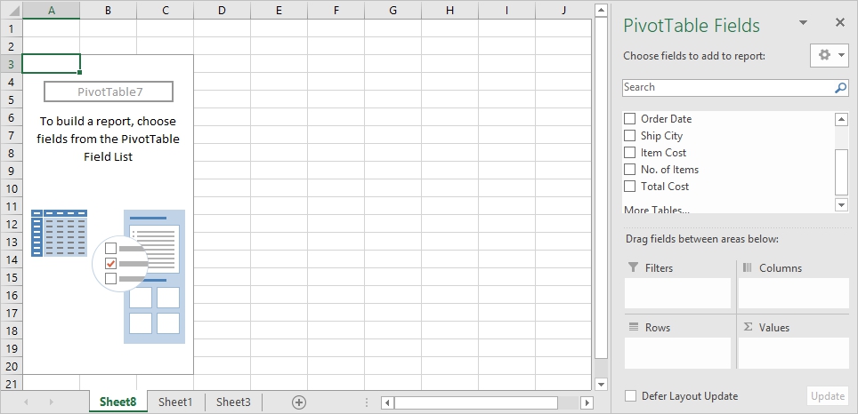
A new worksheet will now be created with a PivotTable placeholder, and on the right side, you'll see a dialog box - PivotTable Fields .

The PivotTable tool has four areas where you can place fields:

Rows , Columns , Values , and Filters .

To add a field to your PivotTable, select the checkbox next to the field name in the PivotTable Fields pane. When you select fields, they are added to their default areas. Non-numeric fields are added to the Rows box. Date and time fields are added to the Columns box. Numeric fields are added to the Values box.

You can also drag fields from the list to one of the four areas you want to place it. To move one field to another, you can drag it there.

To remove a field from a box, click on it and click Remove Field from the pop-up menu. You can also just uncheck it in the fields list or drag it away from the box and drop it back on the fields list.

Example

In this example, let's say we want a summary of our data that shows the total spent by each Customer.

1. Select the Customer field on the list and it will be added to the Rows box. The PivotTable will also be updated with the list of customers as row headings.
2. Next, select the Total Cost field and this will be added to the Values box.

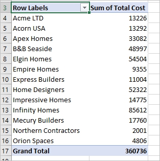
The PivotTable will now be updated with the Sum of Total Cost for each Customer.

So, as you can see, we have been able to get a quick summary of our data with just a few clicks. If we had hundreds of thousands of records, this could have taken many hours to accomplish, if done manually.

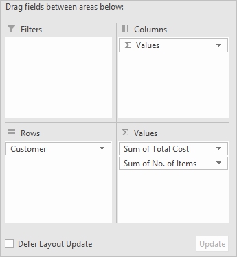
We can add more values to the table by dragging them to the Values box from the list.

For example, if we wanted to add the total number of items per customer, we'll select No. of Items on the list or drag it to the Values box.

This will add the Sum of No. of Items for each customer to the PivotTable as shown in the image below.

To view the summary from the perspective of Products , i.e. the total number of items sold and the total cost for each product, we would put Product in the Rows box and both Total Cost and No. of Items in the Values box.

To view the summary from the perspective of Employees , we would place Employee in the Rows box, and No. of Items and Total Cost in the Values box.

Here we see the data summarised by Employee i.e. how many items each employee sold, and the revenue generated.

If we want to see the number of items sold per city, we would place Ship City in the Rows box and No. of Items in the Values box.

Summarising Data by Date

To display the columns split into years, drag a date field into the Columns box, for example, Order Date. The PivotTable tool will automatically generate PivotTable fields for Quarters and Years. Once these fields have been generated, you should remove the Order Date field from the Columns box and place in the Quarter or Year field, depending on which one you want to use for your summary.

To display the row headings by date, place Order Date (or your date field) in the Rows box.

This will produce the following results.

Applying Formatting

As you can see, we can dynamically change how we want to view our data with just a few clicks. When you're happy with your summary, you can then apply formatting to the appropriate columns. For example, you could format Sum of Total Cost as Currency before any formal presentation of the data.

The good thing about PivotTables is that you can explore different types of summaries with the pivot table without changing the source data. If you make a mistake that you can't figure out how to undo, you can simply delete the PivotTable worksheet and recreate the PivotTable in a new worksheet.