Generate a PivotTable and a PivotChat Simultaneously

You can generate a pivot table and a pivot chart simultaneously from your data list without having to generate the pivot table first.

To generate the pivot table and pivot chart together, do the following:

1. Click anywhere in the data list.
2. On the Insert tab click the drop-down arrow for the PivotChart command button.
3. Select PivotChart & PivotTable from the drop-down menu on the command button.
4. On the Create PivotTable dialog box, click the OK button.

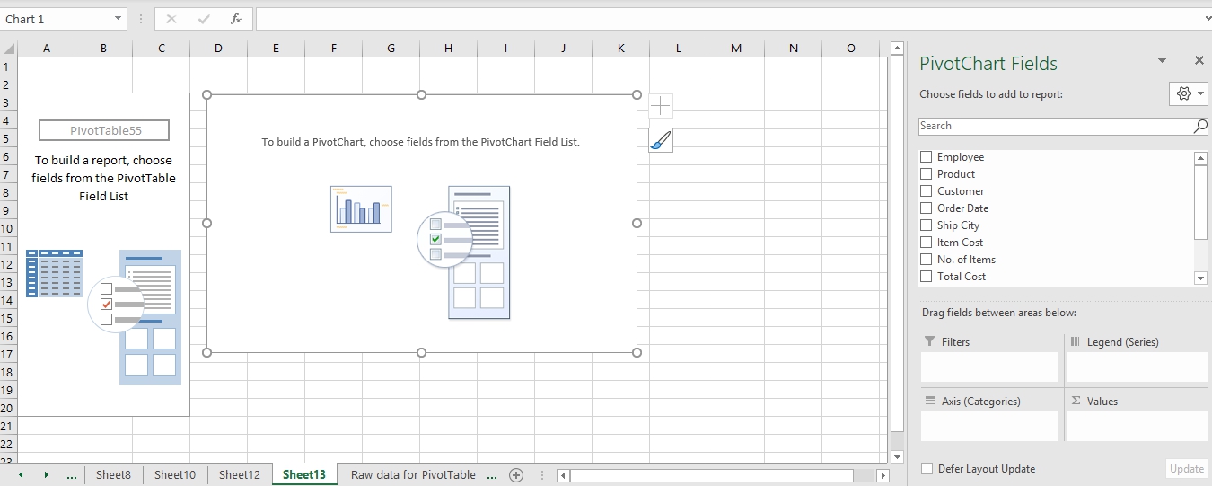
Excel will create a new worksheet with the placeholders for a pivot table and a pivot chart. In the PivotChart Fields pane on the right side of the window, you can select the fields to go in your pivot chart, just as described in the section on manually creating a PivotTable in this chapter. As you select the fields you want for the chart in the PivotChart Fields pane, the pivot table and pivot chart will be created together.

Formatting a PivotChart

Formatting a pivot chart is similar to formatting a regular Excel chart, which I covered in my Excel 2019 Basics book. If you want to learn how to edit and format charts, I recommend looking up the chapter, Creating Charts in my Excel 2019 Basics book.