Protect Specific Ranges

When you protect a worksheet, by default Excel locks all cells, unless you specifically unlock some cells before you enable protection (as described above). If all cells are locked, then to access the locked parts of the sheet you have to remove the sheet protection altogether.

What if we have occasions where we want to enable some users to have access to locked ranges without removing the sheet protection?

Excel provides a solution with the Allow Edit Ranges command. You can password protect specific ranges in the worksheet rather than the whole sheet.

Also, if you’re using a Microsoft Windows machine that is on a network domain, you can give specific users in your domain permission to edit ranges in a protected worksheet.

The process involves two steps:

1. Specify the ranges to be password protected.
2. Protect the worksheet.

Step 1 - Follow these steps to specify the ranges to be password protected:

1. If the worksheet is already protected, you need to unprotect the sheet first.
2. Select the worksheet that you want to protect by clicking on the sheet tab at the bottom of the screen.
3. On the Review tab, in the Protect group, click Allow Edit Ranges . Note that this command button is only available when the worksheet is unprotected.
   
4. To add a new range that you want to be editable using a password, click New .
   
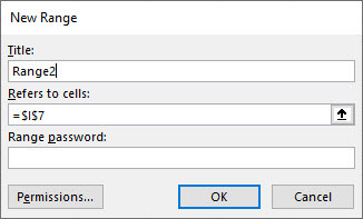
5. On the New Range dialog box, in the Title field, type the name for the range that you want to unlock.
6. In the Refers to cells field, you can type in the cell reference of the range, starting with an equal sign (=). Alternatively, you can click on the Collapse Dialog button (the up arrow on the field) and select the range on the worksheet. Click the Collapse Dialog button again to return to the New Range dialog box.
7. In the Range password field, enter a password that allows access to the range.
   Note : To use domain permissions, click the Permissions button and follow the process to add a domain user. This only applies to network domains with multiple user accounts.
8. Click OK to return to the Allow Users to Edit Ranges dialog box.

Step 2 - Protect the worksheet:

1. In the Allow Users to Edit Ranges dialog box, click the Protect Sheet button.
   Note : If you have closed the Allow Users to Edit Ranges dialog box, then click Protect Sheet on the Review tab of the Ribbon.
   
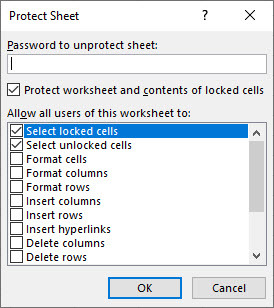
2. The Protect worksheet and contents of locked cells check box should be selected by default. If it is not you should select it.
3. In the Allow all users of this worksheet to list, select the actions you want users to be able to carry out on the worksheet. For example, you could allow users to insert rows and columns, sort data, format cells, or use AutoFilter, among the many options on the list.
4. In the Password to unprotect sheet field, enter a password and Click OK . Re-enter the password to confirm it and click OK again.

As mentioned previously, the password is optional. If you don’t set a password, any user can click the Unprotect Sheet button on the Ribbon to unprotect the sheet.

Once a range has been protected, the user will be prompted to enter a password when they try to edit it. They’ll only need to enter the password once per session.

Important! This has been mentioned earlier in this chapter but is worth repeating. If you set a password to protect your worksheet, you’ll need the password whenever you want to unprotect it. Hence, it is critical that you remember your password. Ideally, you want to have it written down somewhere under lock and key for easy retrieval if needed. If you forget the password there are no tools provided by Microsoft to retrieve it.