CHAPTER 31
Basic statistics: Assessing the impact of a diagnostic test; choosing a gold standard, sensitivity, specificity, PPV, NPV, and likelihood ratios
Stephen R. Hayden
Department of Emergency Medicine, UC San Diego Health Systems, CA, USA
Diagnostic tests rarely establish the presence of a medical condition with certainty; instead, a physician uses test results to help strengthen their estimate that a disorder is either likely or less likely in an individual patient [1]. If a test is not going to inform decision making in this manner, clinicians should question why it is necessary to obtain it in the first place.
Our estimate of disease probability before knowing the result of a diagnostic test is called the pretest or prior probability and the estimate after knowing the test result is termed the post-test or posterior probability of disease. The degree to which pretest probability is modified to obtain an estimate of post-test probability is determined by the characteristics of the test. These characteristics are classically measured and reported in a number of ways and provide an idea of the impact the results of a diagnostic test will have on your clinical decision making. In this chapter the following characteristics of diagnostic tests are discussed as they commonly apply to acute care research:
- Sensitivity
- Specificity
- Accuracy
- Positive and negative predictive value
- Likelihood ratio.
Before considering these elements, however, it is worth mentioning what we mean by a “gold” standard. When designing or appraising a study on how good a particular diagnostic test is at distinguishing between patients that have the disease of interest and those that do not, the test needs to be compared to a standard or criterion that reasonable clinicians would agree makes the definitive diagnosis or defines the target disorder [2]. In other words, the accuracy of a diagnostic test is best determined by comparing it to the “truth” or as close to it as we can come. It is likewise important that ALL subjects that have the test of interest performed also have the gold (or “criterion”) standard test completed [2]. This may not always be as straightforward as it seems. For example, in the early studies of the utility of computed tomography (CT) scanning for appendicitis, findings on CT were compared to presence of inflammation on the pathological specimen removed at operation. However, it is not only impractical but also unethical to design a study that unnecessarily subjects some patients to surgery they may not need. These early studies included only those patients already selected for surgery and so represented a skewed patient population (selection bias). The true practical value of a test is established only in a study that closely resembles clinical practice and not just patients with severe disease. It is important to include an appropriate number of patients and spectrum of disease to assess the test in real life circumstances. Later studies looking at CT in appendicitis used a combined outcome of surgical pathology results or clinical follow up at 30–90 days as a criterion standard against which to compare CT results.
There are two other important aspects to consider when designing a study to evaluate a diagnostic test. Firstly, the interpretation of both the criterion standard as well as the new test should be independent and blinded to important clinical information or outcome [2]. This is especially important for tests that require integration or analysis such as radiological imaging. Secondly, the results of the test being evaluated cannot influence the decision to perform the criterion standard for comparison [2], otherwise the properties of the test will be artificially inflated; this is called verification bias. An example of this would be a study on patients with suspected acute coronary syndrome and exercise stress testing where patients with positive stress testing are more likely to undergo angiography (criterion standard) than those with negative stress testing.
Test results when two outcomes are possible
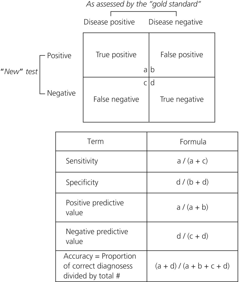
In the acute care setting, diagnostic tests are often reported as “positive” or “negative” (binary outcomes), even if the actual data represent a number on a continuous scale. In the latter case a cutoff point is chosen above which the result is considered positive, below which it is negative; this is called dichotomization of continuous data. An example is quantitative D-dimer testing for pulmonary embolism in which a cutoff point of 500 μg/L is used for a commonly performed assay in patients under age 50 years. When results are reported this way, test characteristics can be described using sensitivity, specificity, positive predictive value (PPV), and negative predictive value (NPV). These values are simple to calculate and understand using a classic 2 × 2 table (Figure 31.1).

Figure 31.1 A 2 × 2 Table for a diagnostic test.
Sensitivity and specificity
Sensitivity is the ability of a diagnostic test to reliably predict the presence of disease. It answers the question, “Of all people who have disease, what proportion is test positive?” Mathematically, it is calculated as the true positives divided by the sum of the true positives plus false negatives, or from the 2 × 2 table: a / (a + c). It is sometimes referred to as a “vertical” property of a 2 × 2 table, meaning that the values do not vary significantly with changes in the prevalence of disease in the population, whereas the positive and negative predictive values do. Specificity refers to the ability of a test to reliably predict the absence of disease. It answers the question, “Of all people who do not have disease, what proportion is test negative?” It is calculated as the true negatives divided by the sum of the true negatives plus false positives, or from the 2 × 2 table: d / (b + d). Like sensitivity, specificity is also referred to as a vertical property and does not vary much with prevalence of disease.
Two rules of thumb that are useful to remember in applying sensitivity and specificity are SPin and SNout. SPin refers to the situation in which a test with a very high specificity can help the clinician “rule in” disease if the result is positive, while SNout refers to the circumstance where a test with a very high sensitivity can help “rule out” disease if the test result is negative.
Take the example of a 23-year-old woman who presents with shortness of breath and non-productive cough for one day. She is otherwise healthy, denies chest pain except when she coughs, and takes no medications other than birth control pills. She has no recent immobilization or surgery, no history of deep vein thrombosis (DVT) or pulmonary embolus (PE), no history of cancer, and her examination is normal including normal oxygen saturation and no signs of a DVT. You feel she has a low probability of PE but cannot completely exclude it as a possibility. Consequently, you wonder if a D-dimer would help inform your clinical decision making. In this situation, you want to modify your estimate of pretest probability from low to extremely low; so low, in fact, that no further work-up is necessary and you can exclude PE in favor of an alternate diagnosis. This would require that D-dimer have a very high sensitivity (SNout). You are able to locate a very recent systematic review in the British Medical Journal from 2013 in which the pooled sensitivity from over 5500 patients in the age group less than 50 years is 97.6 (95% CI: 95.0–98.9) and feel confident that a negative D-dimer in your patient would exclude a PE [3].
Positive and negative predictive value
The positive predictive value (PPV) of a test relates to how likely a test will be positive when disease is truly present. PPV helps answer the question, “Of all the people who are test positive, what proportion will actually have the disease?” and is calculated as the true positives divided by the sum of the true positives plus the false positives, a / (a + b). Likewise, the negative predictive value (NPV) of a test reflects how likely a test will be negative when disease is truly absent. NPV helps answer the question, “Of all the people who are test negative, what proportion will not have the disease?” and is calculated as the true negatives divided by the sum of the true negatives plus the false negatives, d / (c + d). PPV and NPV are sometimes termed horizontal properties of the 2 × 2 table and ultimately vary with the prevalence of disease in a population of patients.
Accuracy of a diagnostic test
The accuracy of a diagnostic test refers to its overall ability to predict both the presence and absence of disease. It is calculated as the sum of the true positives plus the true negatives divided by the total. Interestingly, this measure of a test is often not reported in many research studies; most probably because it loosely combines sensitivity and specificity, which often have an inverse relationship. In other words, in studies where continuous data are being dichotomized and a cutoff point is being determined, one must sacrifice sensitivity in order to maximize specificity and vice versa.
Likelihood ratio
Is your head swimming yet? If so, you are not alone. These concepts are not intuitive for clinicians in the acute care setting. While we are familiar with the terms sensitivity, specificity, NPV, and PPV, discussions about true positives, false negatives, and how NPV varies with disease prevalence are not practical at the bedside. Another disadvantage to these measures is that they can only be used in situations where test results are binary. For tests in which more than two results are possible, sensitivity, specificity, PPV, and NPV are no longer applicable. A classic example of this is the ventilation perfusion lung scan (or VQ scan) for pulmonary embolism. Results from this test are often reported as normal, low probability, intermediate, or high probability, and so do not fit neatly in a 2 × 2 table as in Figure 30.1. A Likelihood Ratio (LR), however, does not suffer from this limitation and can be calculated and applied to any test result, whether binary, multiple, interval, or continuous data.
A LR also allows a clinician to more directly estimate post-test probability from pretest probability of disease. For many clinicians it is a more intuitive measure of the impact of a diagnostic test and helps answer the important question, “What are you going to do with the result of that test?”
Likelihood ratio for dichotomous test results
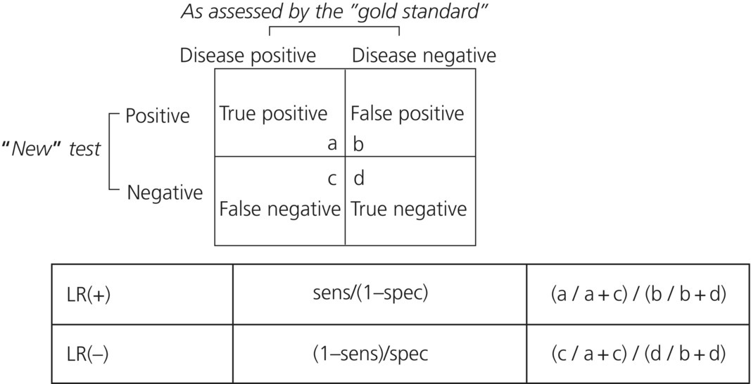
In the situation where two test results are possible, usually reported as positive or negative, the LR is referred to as either the LR positive or LR negative. The LR(+) is the probability of a positive test result in patients with disease divided by the probability of a positive test result in patients without disease [1]. It is the probability of the test result, NOT the probability of disease! Similarly, the LR(–) is the probability of a negative test result in patients with disease divided by the probability of a negative test result in patients without disease.
Mathematically, LRs can be calculated from a 2 × 2 table just like other measures of diagnostic tests and should be reported in studies evaluating a new diagnostic test or strategy (Figure 31.2).

Figure 31.2 2 × 2 Table; likelihood ratios.
Rules of thumb [1]
- LR of 1 means test result does not change probability of disease = no impact.
- LR of 2–5 or 0.5–0.2 = modest impact on clinical decision making.
- LR of 5–10 or 0.2–0.1 = moderate impact.
- LR of >10 or <0.1 = major impact.
Consider the example of 27-year-old-man presenting to the ED with lower abdominal pain for one day. Initially his pain was poorly localized but now it seems it is worse in his periumbilical region. He denies fever, has mild nausea but no vomiting, and is able to tolerate oral foods but his appetite is diminished. He has a history of kidney stones but states this is different. His vital signs are normal and his examination is normal except for mild tenderness to palpation in the midline, lower abdominal area without overt rebound tenderness or guarding. You order a urinalysis and laboratory tests and suggest that an abdominal CT be obtained. The patient expresses concern that he has already had two CT scans in the past two years for recurrent kidney stones and asks if an ultrasound (US) might be an alternative?
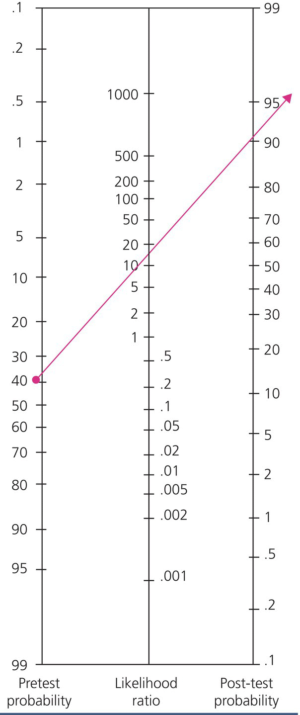
In order to answer this question, you need to know the test characteristics of US for the diagnosis of suspected appendicitis in the acute care setting and what impact it would have on your estimate of this patient’s pretest probability of appendicitis. This is easily answered by knowing the LR(+) and LR(–) of US for appendicitis in patients presenting to the ED with abdominal pain. In a multicenter study published in Radiology in 2013 by Leeuwenburgh et al., the reported sensitivity and specificity of graded compression US was 77% and 94% respectively, the LR(+) was 12 and the LR(–) was 0.25 [4]. Knowing the sensitivity and specificity in this case does not help you as much in your clinical decision making. You estimate your patient’s pretest probability of appendicitis is in the low to moderate range, therefore the sensitivity is not high enough to rule out disease without further information or testing, and the specificity of 94% does not necessarily “rule in” disease with enough precision. However, starting from a low to moderate pretest probability of approximately 40%, if the US is positive for appendicitis, knowing the LR(+) is 12 allows a direct estimate of post-test probability of 90% using a simple nomogram [5], (Figure 31.3). Given the clinical scenario, and a probability of appendicitis of 90% or more, most surgeons would take this patient to the operating room. Conversely, if the US is negative, a LR(–) of 0.25 means his post-test probability of appendicitis is still 10–12% and further testing is necessary. Interestingly, in the same study by Leeuwenburgh et al., immediate MRI was compared to the criterion standard if US was negative and the LR(+) for MRI was 15, and LR(–) was 0.04 [4].

Figure 31.3 Fagan Nomogram5.
Likelihood ratios for interval or continuous data
By nature, most laboratory information is quantitative. Interpretation, therefore, often depends on the degree of positivity or negativity of a result, not just qualitatively whether the result is positive or negative alone. Grouping together quantitative data into two arbitrary groups based on a cutoff point loses both information and the ability to more precisely discriminate between groups. Intuitively, though, clinicians would agree that there is a difference in likelihood that a PE is present in a patient with a D-dimer of 501 and a D-dimer of 5000, when 500 is used as the level to define positivity.
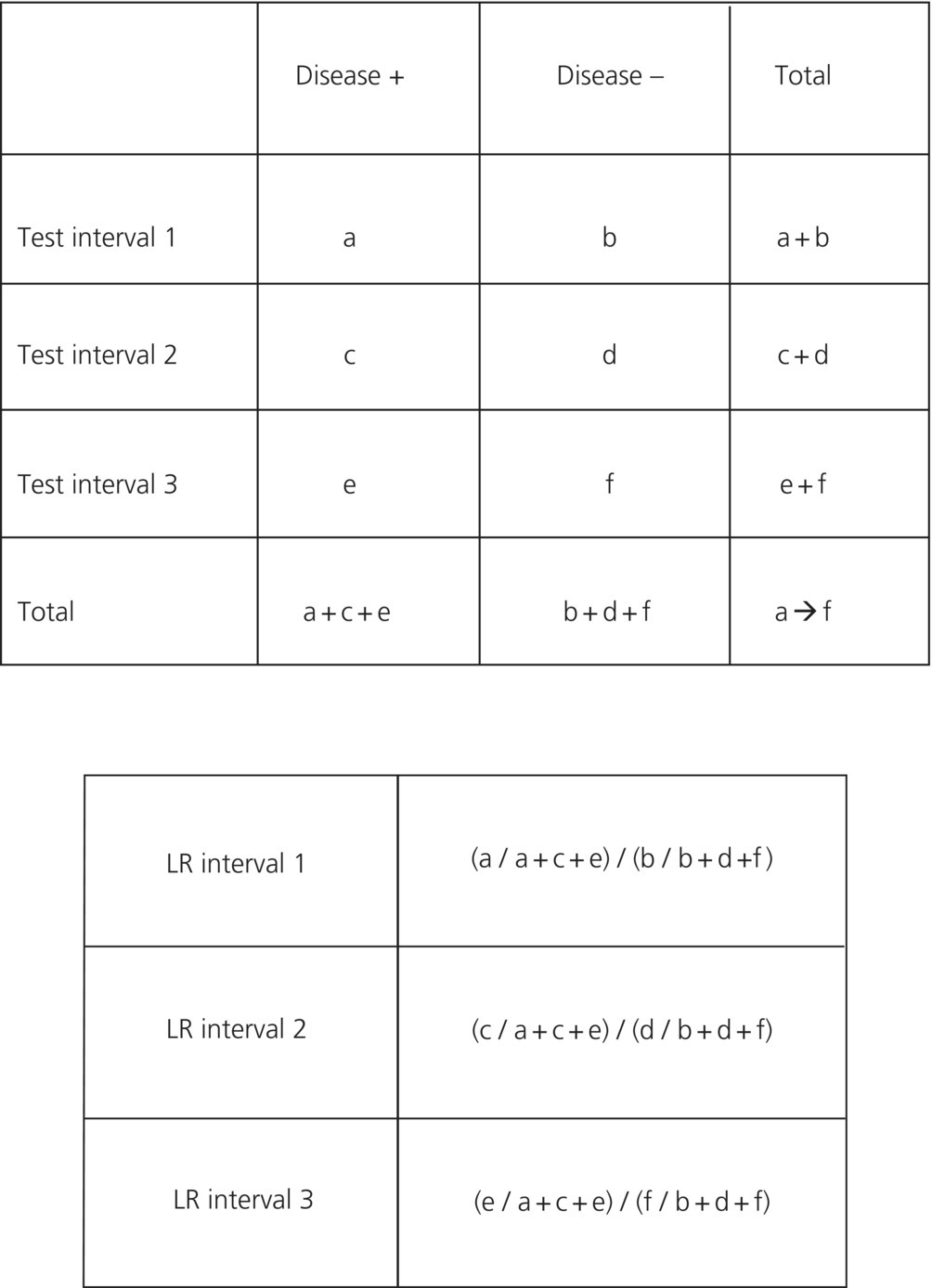
Likelihood ratios can be calculated for test results that are reported in any number of intervals, but it is most useful to define the intervals in such a way to stratify patients into groups where decisions make clinical sense. A classic example might be a test that reports results in terms of low probability/risk, moderate risk, or high risk such as a VQ scan. Intervals can be defined and a contingency table can be set up as in (Figure 31.4).

Figure 31.4 Calculating interval likelihood ratios.
References
- 1 Hayden, S.R. and Brown, M.D. (1999) Likelihood ratio: A powerful tool for incorporating the results of a diagnostic test into clinical decision making. Ann Emerg Med, 33:575–580.
- 2 Jaeschke, R., Guyatt, G.H., Sackett, D.L., et al. (1994) User’s guides to the medical literature, III: How to use an article about a diagnostic test. JAMA, 271:703–707.
- 3 Schouten, H.J., Geersing, G.J., Koek, H.L., et al. (2013) Diagnostic accuracy of conventional or age adjusted D-dimer cut-off values in older patients with suspected venous thromboembolism: systematic review and meta-analysis. BMJ, 346:f2492.
- 4 Leeuwenburgh, M.M., Wiarda, B.M., Wiezer, M.J., et al. (2013) Comparison of imaging strategies with conditional contrast enhanced CT and unenhanced MR imaging in patients suspected of having appendicitis: A multicenter diagnostic performance study. Radiology, 268(1):135–143.
- 5 Fagan, T.J. (1975) Nomogram for Baye’s theorem (C). N Engl J Med, 293:257.