A. Scozzari et al. (eds.)ICT for Smart Water Systems: Measurements and Data ScienceThe Handbook of Environmental Chemistry102https://doi.org/10.1007/698_2019_403
Exploring Assimilation of Crowdsourcing Observations into Flood Models
M. Mazzoleni1, 2, Leonardo Alfonso3 and D. P. Solomatine3, 4
(1)
Department of Earth Sciences, Uppsala University, Uppsala, Sweden
(2)
Centre of Natural Hazards and Disaster Science (CNDS), Uppsala, Sweden
(3)
IHE Delft Institute for Water Education, Delft, The Netherlands
(4)
Delft University of Technology, Delft, The Netherlands
This chapter aims to describe the latest innovative approaches for integrating heterogeneous observations from static social sensors within hydrological and hydrodynamic modelling to improve flood prediction. The distinctive characteristic of such sensors, with respect to the traditional ones, is their varying lifespan and space-time coverage as well as their spatial distribution. The main part of the chapter is dedicated to the optimal assimilation of heterogeneous intermittent data within hydrological and hydraulic models. These approaches are designed to account for the intrinsic uncertainty contained into hydrological observations and model structure, states and parameters. Two case studies, the Brue and Bacchiglione catchments, are considered. Finally, the evaluation of the developed methods is provided. This study demonstrates that networks of low-cost static and dynamic social sensors can complement traditional networks of static physical sensors, for the purpose of improving flood forecasting accuracy. This can be a potential application of recent efforts to build citizen observatories of water, in which citizens not only can play an active role in information capturing, evaluation and communication but also can help improve models and increase flood resilience.
The impact of natural hazards on societies and economies has drastically increased in the last years due to many natural and anthropogenic factors, including climate change [1, 2]. For this reason, the demands for non-structural measures able to accurately and timely forecast in real-time river water level to allow decision-makers to take the most effective and timely decisions for reducing harm or loss have significantly increased [3–5]. Among different types of water system models, hydrological and hydrodynamic models are the most utilised ones in flood early warning systems in river basins.
Unfortunately, deterministic predictions contain an intrinsic uncertainty due to many sources of error that propagate through the model and therefore affect its output [6]. In fact, uncertainty can be due to either the inherent stochastic nature and variability of hydrological processes, i.e. aleatory uncertainty [7, 8], or to our imperfect state of knowledge of the hydrological system and our limitedness to model it, i.e. epistemic uncertainty [9–12]. Three main sources of uncertainty can be identified [13] in hydrological and hydrodynamic modelling: (a) observation uncertainty, which is the approximation in the observed hydrological variables used as input or calibration data (e.g. rainfall, temperature and river discharge); (b) parameter uncertainty, which is induced by imperfect model calibration; and (c) model structural uncertainty, which is a result of the inability of models to perfectly schematize the physical processes involved. Epistemic uncertainty can be associated with the latest two sources of uncertainty previously mentioned due to limited knowledge about the physical behaviour of the system.
A reliable characterisation and reduction of the uncertainties affecting hydrological and hydrodynamic processes is an important scientific and operational challenge [14–17]. Different approaches like the first-order reliability method [18], probabilistic Monte Carlo (MC) and fuzzy rule-based methods [19–21] can be used to assess model uncertainty.
Several research activities aimed to reduce such uncertainty in the flood estimation, predictive uncertainty, have been carried out due to its importance to the decision of issuing a flood warning [5, 22, 23]. Methods like the UNcertainty Estimation based on Local Errors and Clustering (UNEEC, [24–26]), Generalised Likelihood Uncertainty Estimation (GLUE, [27, 28]) and Machine Learning in parameter Uncertainty Estimation (MLUE, [29, 30]) can be employed to assess uncertainty in water system models and estimate predictive uncertainty (see, e.g. [31, 32]). However, such tools are often not used in operational forecasting by environmental agencies and river basin authorities, perhaps because of their belief that uncertainty analysis cannot be incorporated into the decision-making process and because uncertainty analysis is too subjective, among others [5, 11, 33].
In the last decades, model updating techniques for reducing predictive uncertainty approaches have been increasingly studied and implemented in water-related applications. These approaches allow for changing model input, states, parameters or output in response of new observations coming into the model in order to improve the prediction accuracy and quantifying uncertainty [3, 14, 34]. In most of the cases, model updating occurs only in form of data assimilation using information of streamflow, soil moisture, etc. coming from static physical stations. Model updating techniques are rarely implemented in operational forecasting due to the lack of approaches to quantify the uncertainty in real-time observations from multiple sources across a range of spatiotemporal scales and methods to integrate these new information in an appropriate and transparent way. In this respect, in operational practice it is preferred to correct the model inputs (in most of the cases), states, initial conditions and parameters in an empirical and subjective way rather than apply advanced (optimal) data assimilation techniques for improving hydrologic forecast [35]. Welles et al. [36] and Liu et al. [34] pointed out how the need for implementing reliable data assimilation methods in operational forecast is increasing in order to fill the mentioned gap with the scientific world.
Traditionally, static physical sensors, such as pressure sensors, water level sensors, and pluviometers, are commonly used by water authorities to calibrate, validate and (in some cases) update physical models in real time. However, the main problem of physical sensors is the proper maintenance which can be very expensive in case of a vast network as well as the limited data that existing sparse monitoring networks can provide to this end.
The continued technological advances have stimulated the spread of low-cost sensors that has triggered crowdsourcing as a way to obtain observations of hydrological variables in a more distributed way than the classic static physical sensors [37]. The main advantage of using these types of sensors is that they can be used not only by technicians, as is the case of traditional physical sensors, but also by regular citizens. Recently, citizen science activities have been widely promoted in order to allow citizens to participate in different aspects of environmental planning and management. One of the most common activities to achieve such goal includes involving citizens in data collection, or crowdsourcing (CS). In particular, observations of hydrological variables can generate additional knowledge, in relation to the water cycle, and use such knowledge in decision-making [38, 39]. However, because of their relatively limited reliability, and random accuracy in time and space, crowdsourced observations have not been widely integrated in hydrological and/or hydraulic models for flood forecasting applications. Instead, they have generally been used to validate model results against observations, in post-event analyses. Different studies addressed the issue of assimilation of distributed observations in distributed and semi-distributed hydrological models (e.g. [40–43]). Neither of the previous studies considers the dynamic nature of data from heterogeneous sensors which provide an intermittent signal in time and space. In fact, the information coming from a specific sensor might be sent just once, occasionally or in time steps that are non-consecutive, i.e. with intermittent observations having different lifespans.
A number of studies have developed methods for using crowdsourced citizens-based observations in water-related models [44–56]. In particular, crowdsourced information are used for directly creating deterministic or probabilistic flood maps [48], derive stream discharges and flow velocities fields [57] and flood extent [52]. In alternative, crowdsourced data have been used for validating flood models [44, 56]. A detailed review on the use of citizen observations for flood modelling applications is provided in Assumpção et al. [58]. However, none of the previous studies assessed the usefulness of citizen observations for improving flood predictions [39, 59]. The first attempts to study the effects of assimilating crowdsourced citizen observations in hydrological and hydraulic models for improving flood prediction in real-time applications are reported in Mazzoleni et al. [60–62] and Mazzoleni [63]. Just recently, Mazzoleni et al. [64] proposed two innovative approaches to assimilated qualitative flow data within hydrologic routing models.
In this chapter, we describe the proposed innovative methods to assimilate heterogeneous intermittent observations, coming from social sensors, within hydrological and hydrodynamic modelling to improve flood prediction. This research was carried out under the framework of the European project WeSenseIt (https://www.wesenseit.com/) [65].
2 Crowdsourced Observations
In this chapter, we consider two different types of sensors to measure hydrological variables such as water level: static physical (StPh) and static social (StSc) sensors (see Fig. 1). In addition, also dynamic social sensors may be used but are not included in this chapter. An example of a static social sensor is a staff gauge located in a strategic point of the river used by citizens to estimate water depth values using a mobile phone app to send CS observations using the QR code as geographical reference point. An example of dynamic sensor is a mobile app allowing any citizen to send the information related to the distance between the water profile and the river bank using a mobile app at random locations along the river. It might be in fact difficult to estimate the water depth value without having any indication about river depth. In this case, the CS observations have higher degree of uncertainty due to the indirect method used to estimate water depth value.
Fig. 1
Proposed sensors classification with (a) static physical sensors (StPh), (b) static social sensors (StSc), and (c) dynamic social sensors (DySc)
According to the nature of the sensor, uncertainty can be defined either as a probability distribution (quantitative observation) or a fuzzy set (qualitative or semi-qualitative observations).
During the last decades, probability theory has been applied in order to represent epistemic or observational uncertainty in mathematical models. In particular, quantitative observations of physical variables can be expressed as a stochastic variable with a given probability distribution which represents the likelihood of that variable value to take on a given value. In most of the cases, stochastic variables are represented using a normal distribution with assigned mean and standard deviation. The higher is the standard deviation, the higher the uncertainty of that variable is.
Examples of qualitative information can be found in verbal or text messages coming from social networks (Twitter, Facebook, etc.). Fuzzy logic emerged as a more general form of logic that can handle the concept of possibilistic values or partial truth. This approach has been used recently [64] as a qualitative modelling methodology since it allows for an easier transition between human and computers for decision-making (transition from fuzzy to numerical data), and it is able to handle imprecise and uncertain information [66]. From a statistical point of view, a physical variable can be associated to a deterministic value plus a given degree of uncertainty, expressed as a pdf, or the second or third order moment. In fuzzy logic-based approach, a physical variable value (e.g. precipitation) would belong to a specific fuzzy set having given characteristic (e.g. low, medium, high precipitation).
3 Case Studies and Water-Related Models
Two different case studies having different hydrometeorological characteristics are analysed in this book chapter. The case studies are the Brue catchment (UK) and the Bacchiglione catchment (Italy). Different hydrological and hydraulic models are implemented within each case study. In particular, a semi-distributed version of a continuous Kalinin-Milyukov-Nash (KMN) cascade hydrological model is applied on the Brue catchment, while a semi-distributed hydrological and hydraulic model developed by the Alto Adriatico Water Authority is implemented in the Bacchiglione catchment. In this study, synthetic flow observations derived from observed and simulated quantitative streamflow are used. Synthetic data are used to evaluate the potential of the proposed approaches as real qualitative observations may be affected by different unpredictable errors.
3.1 Brue Catchment (UK)
The Brue catchment is located in Somerset, South West England, with a drainage area of about 135 km2 and a time of concentration of 10 h at the catchment outlet, Lovington. Hourly precipitation data are supplied by the British Atmospheric Data Centre from the NERC Hydrological Radar Experiment Dataset (HYREX) project [67, 68] and available at 49 automatic rain stations; average annual rainfall of 867 mm is measured in the period between 1961 and 1990. Discharge is measured at the catchment outlet by one station at a 15 min time step resolution, having an average value of 1.92 m3/s. For both precipitation and discharge data, a 3-year complete data set, between 1994 and 1996, is available.
A semi-distributed hydrological model is used to assess the flood hydrograph at the outlet section of the Brue catchment and to represent the spatial variability of the CS flow observations. The Brue catchment is divided into 68 sub-catchments having a small drainage area (on average around 2 km2) so that any observation at a random location in a given sub-catchment would provide the same information content that an observation at the outlet of same sub-catchment [60]. For each sub-catchment, a conceptual lumped hydrological model, continuous Kalinin-Milyukov-Nash (KMN) cascade, is implemented to estimate the outflow discharge [69]. The KMN model considers a cascade of storage elements (or reservoirs), assuming that the relation between stage, discharge and stored water volume is linear and that the water storage xt is only a function of the outflow of the reach Qt [60]. Subsequently, the KMN is represented as a dynamic state-space system to apply data assimilation techniques as explained in the previous section. In the case of the linear systems, the discrete state-space system can be represented as follows [69]:
(1)
(2)
where t is the time step, x is vector of the model states (stored water volume in m3), Φ is the state-transition matrix (function of the model parameters n and k), Γ is the input-transition matrix, H is the output matrix and I and z are the input (forcing) and model output, while w and v are the system and measurements errors.
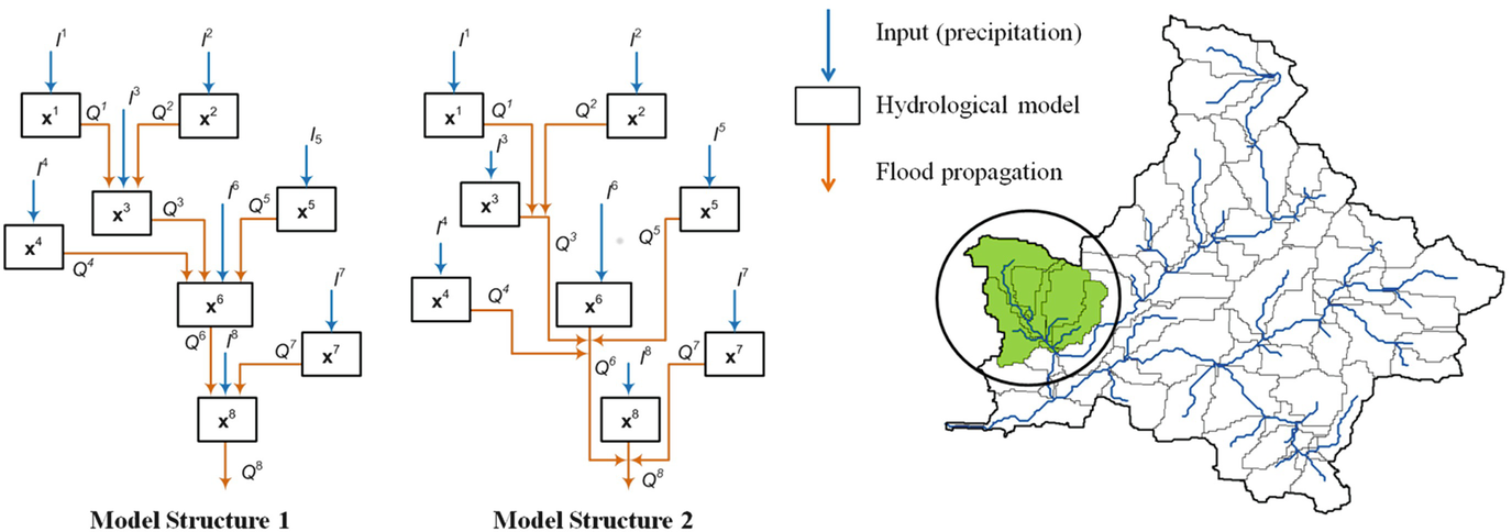
Muskingum channel routing method [70] is used for flow propagation between sub-catchments; for details see Mazzoleni et al. [60]. The semi-distributed model is structured in such a way that the sub-catchments are sequentially connected and the output of the upstream sub-catchments is used as input in the downstream ones (see Fig. 2). More details about the model calibration are reported in Mazzoleni et al. [60].
Fig. 2
Considered model structures (MS) for the semi-distributed hydrological model
3.2 Bacchiglione Catchment (Italy)
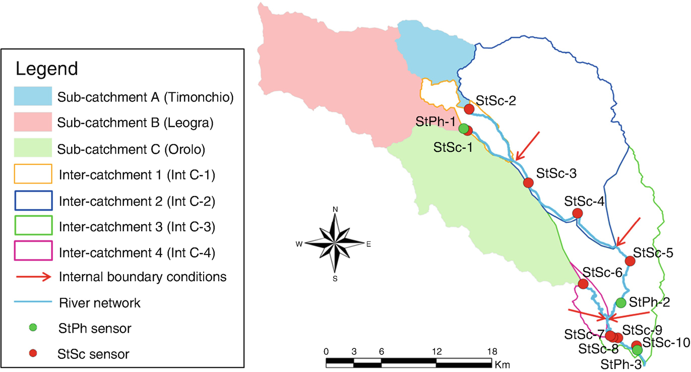
The Bacchiglione River catchment is located in the north-east of Italy and tributary of the River Brenta which flows into the Adriatic Sea at the south of the Venetian Lagoon and at the north of the River Po delta. The considered area is the upstream part of the Bacchiglione River, which has an overall area of about 400 km2, river length of about 50 km, river width of 40 m and river slope of about 0.5% [71]. The main urban area is Vicenza, located in the downstream part of the study area, where recent floods were registered during the springs of 2010 and 2013. Within the activities of the WeSenseIt project [72], one StPh sensor and ten StSc sensors (staff gauges complemented by a QR code, as represented in Fig. 1) were installed in the Bacchiglione River to measure water level (see Fig. 3). Hourly information related to rainfall, temperature, wind direction and intensity, humidity, snow, solar radiation and water level are available for the last 12 years.
Fig. 3
Structure of the semi-distributed model for the Bacchiglione catchment and location of the static physical (StPh) and social (StSc) sensors
In order to represent the distributed hydrological response of this catchment, a semi-distributed model, in which the output of the hydrological model is used as boundary conditions in the hydraulic model, has been implemented.
The hydrological response of the catchment is estimated using the hydrological model developed by the Alto Adriatico Water Authority (AAWA) that considers the routines for runoff generation, having precipitation as model forcing, and a simple routing procedure. The processes related to runoff generation are modelled mathematically by applying the water balance to a control volume, of soil depth, representative of the active soil at the sub-catchment scale. The water content is estimated as function of the precipitation, evapotranspiration, surface runoff, sub-surface runoff and deep percolation. The propagation process in the river channel is represent using a distributed Muskingum-Cunge model discretized each 1,000 m. More details about these models can be found in Mazzoleni et al. [62].
The calibration of the hydrological model parameters was performed by AAWA using an adaptation of the “SCE-UA” algorithm [73], considering the time series of precipitation from 2000 to 2010, in order to minimise the root mean square error between observed and simulated values of water level at PA (Vicenza) gauged station. For the Muskingum-Cunge model, the only parameter that is calibrated in this chapter is the Manning coefficient n, used to estimate the water level along the river. The semi-distributed hydrological-hydraulic model in the Bacchiglione catchment is then validated considering the flood events that occurred in May 2013, November 2014 and February 2016.
In order to apply data assimilation, both the hydrological and Muskingum models are represented using the stochastic state-space form reported in the previous section. In particular, for the Muskingum model, the approach proposed by Georgakakos et al. [74] is used.
4 Model Updating Techniques
Operational forecast can be seen as combination of water models (e.g. hydrological and hydrodynamic) and an updating module. In fact, in the last decades model updating techniques have been intensively used within water system models [75, 76], in order to reduce predictive uncertainty. The hydrological and hydrodynamic models utilise input variables, which are either measured or estimated (e.g. areal precipitation, air temperature, potential evapotranspiration), into a set of equations that contain state variables and parameters. Typically, the parameters remain constant, while the state variables vary in time, even if there are different examples of parameter updating approaches such as Moradkhani et al. [77, 78], Salomon and Feyen [79] and Lü et al. [80]. The feedback process of assimilating the new available information into the forecasting procedure is referred to as updating [75] or DA [76].
The assimilation methods can be divided according to the variables modified during the updating process. In the frequently cited WMO report [76], updating is understood in a wide sense, and input, parameters, states and output updating techniques are distinguished. Recently, Liu et al. [34] provided a detailed review of the status, progresses, challenges and opportunities in advancing DA in operational hydrological forecasting. There are many data assimilation techniques that can be used to integrate hydrological observations within water-related models. In this chapter we will focus mainly on Kalman filter and ensemble Kalman filter.
4.1 Kalman Filter
Kalman filter (KF, [81]) is an approach which allows to optimally estimate the state of a dynamic uncertain model as response of real-time (noisy) observations [3, 14, 77, 82–85]. KF update model states considering only the last available observation allowing for a faster computation. However, KF is optimal only in the case of linear dynamic systems. Kalman filter procedure can be divided in two steps: time update equations, namely, forecast (background) equations, Eqs. (3) and (4),
where x is the nstate × 1 state matrix at time t and t−1, Kt is the nstates× nobs Kalman gain matrix, P is the nstates× nstates error covariance matrix and z0 is the new observation. The superscripts + and – indicate, respectively, the updated and background state values, and Φ and Γ represent the state-transition and input-transition matrices, which change according to the model type and structure. The system and measurement error wt is assumed to be normally distributed with zero mean and covariance R. In the application considered in this chapter, the matrix R is time dependent as the error in the measurement is assumed variable because of the varying behaviour in time and space of the crowdsourcing observations.
A key issue in the implementation of the Kalman filter is the determination of model errors. In fact, an overestimation of model errors can reduce the confidence in the model bringing the KF closer to the observations and vice versa [86]. In this study, the modified version of KF, which accounts for the intermittency of crowdsourced observations in between two model time steps, proposed in Mazzoleni et al. [62] is used.
4.2 Ensemble Kalman Filter
Ensemble Kalman filter [87–90] is a widely used data assimilation method for non-linear dynamic model. The main idea of the EnKF is to represent the forecasted pdf estimate with a set of random samples and estimate the updated probability density function (pdf) of the model states as a combination between data likelihood and forecasted pdf of model states by means of a Bayesian update. In this way, the evaluation of the model error covariance matrix is performed as proposed by Evensen [87]:
(8)
where Nens is the number of ensemble members and E is the ensemble anomaly [40] for each ensemble member:
(9)
where is the ensemble mean. The update states and Kalman gain are calculated using Eqs. (5) and (6). Because the EnKF performance is influenced by the spread of the ensemble [91–93], it is important to properly perturb the system in a way to obtain a reliable spread of the ensemble within a meaningful range [94]. For this reason, in this study we used the approach proposed by Anderson [91] to perturb the system and to evaluate the quality of the ensemble spread. More details are provided in Mazzoleni [63].
In order to implement EnKF, an ensemble of model realisations is generated perturbing the forcing data and the model parameters using a uniform distribution. The observation error is assessed using the approach described in the section below.
4.3 Synthetic Flow Observations
Synthetic flow observations are used because of the lack of distributed crowdsourced observations at the time of this study within the considered case study [62]. Such synthetic observations are generated by two different approaches for the two catchments. On the one hand, for the Brue catchment, the approach used to generate the synthetic values of river flow is very similar to the one used by Weerts and El Serafy [90], in which the model forcing is perturbed by means of a time series normally distributed with zero mean and given standard deviation.
On the other hand, for the Bacchiglione catchment, the observed time series of precipitation are used as input for the hydrological models of the sub-catchments and inter-catchments to generate synthetic discharges and then propagate them with the hydraulic model down to the outlet point of the catchment. In this way, the synthetic WL values at the outlet of the sub-catchments or inter-catchments and at each spatial discretization of the six reaches of the Bacchiglione River are estimated and assumed as observed variables in the assimilation process.
4.4 Estimation of the Observational Error
The correct estimation of the model and observational error is crucial for implementing data assimilation methods. Few studies in the past have addressed this issue (e.g. [95]), but further research is needed. For this reason, we adopted a simplified approach to quantify observational errors. Here, the covariance matrix R is assessed using the approach described in Weerts and El Serafy [90], Rakovec et al. [43] and Mazzoleni [63]:
(10)
where α is a variable related to the accuracy level (i.e. degree to which the measurement is correct overall) of the flow measurement and Qsynth is the synthetic flow observation. In the case of CS observations, accuracy levels vary temporally and spatially.
Table 1 summarises the distribution of the coefficient α of the observational error of Eq. (10). The distribution of the coefficient α does not pretend to be exhaustive in accounting for different inaccuracies of observations coming from physical and social sensors and is subject for further research.
Table 1
Assumed observational errors for the different types of sensors
Sensor type
Assumed accuracy level
Coefficient α
Temporal and spatial variability
Static physical (StPh)
High
α = 0.1
Fixed location
Constant in time
Static social (StSc)
Medium
α = U(0.1, 0.3)
Fixed location
Intermittent arrival
For static social sensors, α values are higher than for static physical sensors and are considered to be a random stochastic variable uniformly distributed in time and space. More details can be found in Mazzoleni et al. [61].
5 Assimilation of Flow Observations from Static Heterogeneous Sensors
This section aims to explore the benefits of assimilating flow observations from a network of static heterogeneous sensors in the case of synchronous (Sect. 5.1) or asynchronous (Sect. 5.2) social observations, depending on the predictability of the arrival time of the observations. In particular, we assume that social sensors provide intermittent observations that can lie either in a specific model time step (synchronous) or in between two model time steps (asynchronous). In addition, social sensors may be distributed within the catchment or be located in a specific point.
5.1 Assimilation of Synchronous Observations
Here, we show the model performance after the assimilation of intermittent synchronous observations, i.e. their arrival time matches the model time step, within the semi-distributed hydrological models of the Brue catchment. We can divide this section in two parts: first, the flow observations are assimilated from different social sensors located within the catchment; second, social sensors are integrated with a network of physical sensors to evaluate the added value of crowdsourced sensors in the assimilation process. A straightforward and pragmatic method (based on EnKF) is used to assimilate the intermittent observations into the hydrological model updating the model states matrix only when observations are available, while when there are no observations, it is assumed that the state covariance error does not change at that time step [60, 96].
5.1.1 Assimilation of Flow Observations Only from Social Sensors
In the first part of this section, we considered MS1 and three different spatial configurations (SC) of static social sensors within the catchments (called scenarios SC1, SC2 and SC3). In particular, SC1 refers to social sensors located along the main river channel, SC2 to sensors located on the upstream part of the main river channel, while SC3 to sensors located close to the catchment outlet. Model results obtaining assimilating flow observations from physical sensors are considered as benchmark in order to compare the assimilation performances using social sensors. A main assumption of this study is that flow observations from social sensors are accepted to be less accurate, with random observation error both in time and space, than the ones from physical sensors.
The difference between the outflow hydrograph estimated assimilating physical and social data (in the same location) is represented in Fig. 4. The different colours of the hydrographs represent the different intermittency configurations of the social sensors, i.e. the unpredictable arrival time of the social observation. The smaller the value of difference, the smaller the sensitivity of the model to assimilation of observations from social sensors. Two different flood events are analysed.
Fig. 4
Differences between assimilation of synthetic physical and social flow data in terms of outflow hydrographs under different intermittency configurations of the social sensors (different colour lines) for MS1 (source [60])
As expected, the assimilation performances change with the different locations of social sensor within the catchment. Considering the flood event A, it can be seen that model outputs are affected by changing from physical to social flow data mainly for SC3. Physically, this can be due to the particular structure of the hydrological model. In particular, the discharge differences in flood event B are smaller than in flood event A due to the different performances of the model without assimilation. In fact, for flood event B, additional real-time observations of discharge slightly improved the model results since the model tends to better estimate the observed value of discharge even without assimilation. It is worth noting that results do not seem to be very sensitive to the intermittency scenarios (different colours of Fig. 4).
The results reported in Table 2 show a large difference in the NSE between assimilations from physical and social sensors. Table 2 underlines that the best model performances are not obtained when the assimilation of flow data is performed using sensors located at the outlet section of the catchment but when sensors are located along the main river channel, i.e. SC1 [60].
Table 2
NSE index values obtained assimilating streamflow observations from different spatial configuration of physical and social sensors for MS1
Spatial configuration
NoDA
1
2
3
Physical sensor
0.46
0.77
0.69
0.75
Social sensors
0.46
0.58
0.51
0.47
5.1.2 Assimilation of Flow Observations from Both Physical and Social Sensors
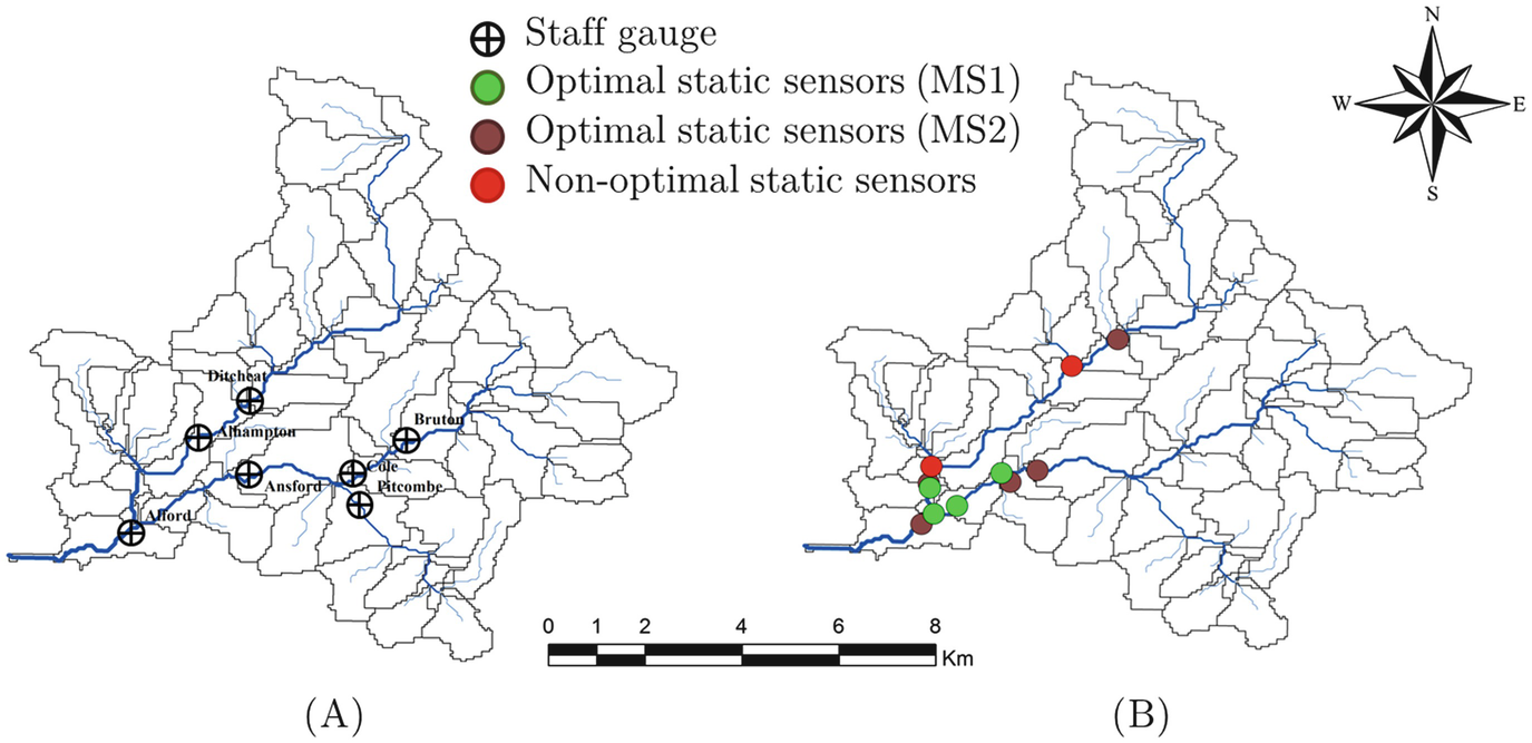
As a matter of fact, the location of the social sensors should typically follow some rules and be subjected to specific constraints. For example, existence of multiple sensors in remote areas of the catchment is quite unlikely due to economical and management reasons. For this reason, in the second part of this section, we assume a realistic configuration of the social sensors closer to the main urbanised area within the catchment (see Fig. 5). The network of social static sensors is integrated with the optimal network of static physical sensors (α equal to 0.1) for MS1 and MS2, respectively.
Fig. 5
Representation of distribution of static physical and social sensors along the Brue Basin for MS1 and MS2, respectively [63]
Different scenarios are introduced based on assumption on the intermittency and availability of CS data and on the possible integration between uncertain CS data and optimal/nonoptimal network of static physical sensors (see Table 3).
Table 3
Description of the different settings
Setting
Social sensors
Physical sensors
Intermittent
Daily timing
Daily and peak timing
Optimal
Nonoptimal
1
–
X
–
–
–
2
X
X
–
–
–
3
–
–
X
–
–
4
X
–
X
–
–
5
–
–
–
X
–
6
–
X
–
X
–
7
X
X
–
X
–
8
–
–
X
X
–
9
X
–
X
X
–
10
–
–
–
–
X
11
–
X
–
–
X
12
X
X
–
–
X
13
–
–
X
–
X
14
X
–
X
–
X
We demonstrate that assimilation of uncertain discharge observations measured at seven staff gauges by social sensors could improve the model results, however, still with the underestimation of the peak flow for scenarios 1 and 2 (see Fig. 6). Assimilation of observations coming from trained volunteers in the time of the peak flow (scenarios 3 and 4) showed a satisfactory improvement of the discharge hydrograph (higher for the model structure 1 than for the structure 2). Intermittent observations do not improve the model results in the same way that social observations coming continuously in time do.
Fig. 6
Outflow hydrographs resulting from the assimilation of physical, social and intermittent observations in the case of realistic scenarios (from a to f) of spatial and temporal distribution of static sensors [63] for MS1 (first row) and MS2 (second row)
Figure 6b confirms that similar improvements for the scenario 3 are achieved assimilating observations coming from the optimally located static sensors running continuously in time (scenario 5). In addition, a combined assimilation of intermittent observations (during daylight time) and static observations from optimal and nonoptimal network of static sensors tends to slightly improve the model output.
Figure 6 demonstrates that considering this type of hydrological model in this particular basin, in the case of an inappropriate distribution of static physical sensors within the basin (scenario 10), the model performances can be improved. However, there is an evident limitation of the model in providing biased hydrographs (especially for MS2), underestimated when compared to the observed one. Biased models can affect the DA results [34].
5.2 Assimilation of Asynchronous Observations
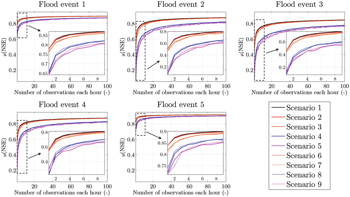
In the previous analysis, social data are provided at the same time of the model time step. However, in case of CS observations, the arrival moment might have lower frequency than the model time step (asynchronous observations), as reported in Mazzoleni et al. [62]. Various experimental scenarios representing different configurations of arrival frequency, number and accuracy of the flow observations are reported in Fig. 7. In order to remove the random behaviour related to the irregular arrival frequency and observation accuracy, different model runs (100 in this case) are carried out, assuming different random values of arrival and accuracy (coefficient α in Eq.10) during each model run, for a given number of observations and lead time. The NSE value is estimated for each model run, so μ(NSE) represents the mean of the different values of NSE.
Fig. 7
The experimental scenarios representing different configurations of arrival frequency, number and accuracy of the streamflow observations [62]
5.2.1 Assimilation of Flow Observations Only from Social Sensors
A lumped hydrological model based on the KMN model is applied to the Brue catchment in order to assimilate synthetic asynchronous observations using the modified version of KF reported in Mazzoleni et al. [62]. Two flood events and experimental scenarios from 1 to 9 (see Fig. 7) are considered in this section.
As it can be seen from Fig. 8, increasing the number of social observations within the observation window results in the improvement of the NSE, but it becomes negligible for more than ten observations. This means that the additional social observations do not add information useful for improving the model performance.
Fig. 8
μ(NSE) values estimated for varying number of assimilated flow observations, for the intermittency scenarios for the different flood events [63]
From Fig. 8 it can be seen that, overall, assimilation of crowdsourced observations improves model performances in all the considered flood events. In the case of scenarios 2 and 3 (represented using warm, red and orange, colours in Fig. 8, for lead time equal to 24 h), i.e. random arrival frequency with fixed/controlled accuracy, the average values of NSE, μ(NSE), are smaller but comparable with the ones obtained in case of scenario 1 for all the considered flood events. In particular, scenario 3 has lower μ(NSE) than scenario 2. This can be related to the fact that both scenarios have random arrival frequency; however, in scenario 3 observations are not provided at the model time step, as opposed to scenario 2. In scenario 4, represented using cold blue colour, observations are considered coming at regular time steps but having random accuracy. Figure 8 shows that μ(NSE) values are lower in case of scenario 4 rather than scenarios 2 and 3. This can be related to the higher influence of observation accuracy if compared to arrival frequency. The combined effects of random arrival frequency and observation accuracy are represented in scenario 5 using a magenta colour (i.e. the combination of warm and cold colours) in Fig. 8. As expected, this scenario is the one with the lower values of μ(NSE) if compared to the previous ones. The remaining scenarios, from 6 to 9, are equivalent to the ones from 2 to 5 with the only difference that they are non-periodic in time. For this reason, in Fig. 8, scenarios from 6 to 9 have the same colour of scenarios 2–5 but indicated with dashed line in order to underline their non-periodic behaviour. Overall it can be observed that non-periodic scenarios have similar μ(NSE) values to their corresponding periodic scenario. However, their smoother μ(NSE) trends are due to lower variability of NSE values which means that model performances are less dependent to the non-periodic nature of the crowdsourced observations than their periodic behaviour. Overall, σ(NSE) tends to decrease for the high number of observations.
5.2.2 Assimilation of Flow Observations from Both Physical and Social Sensors
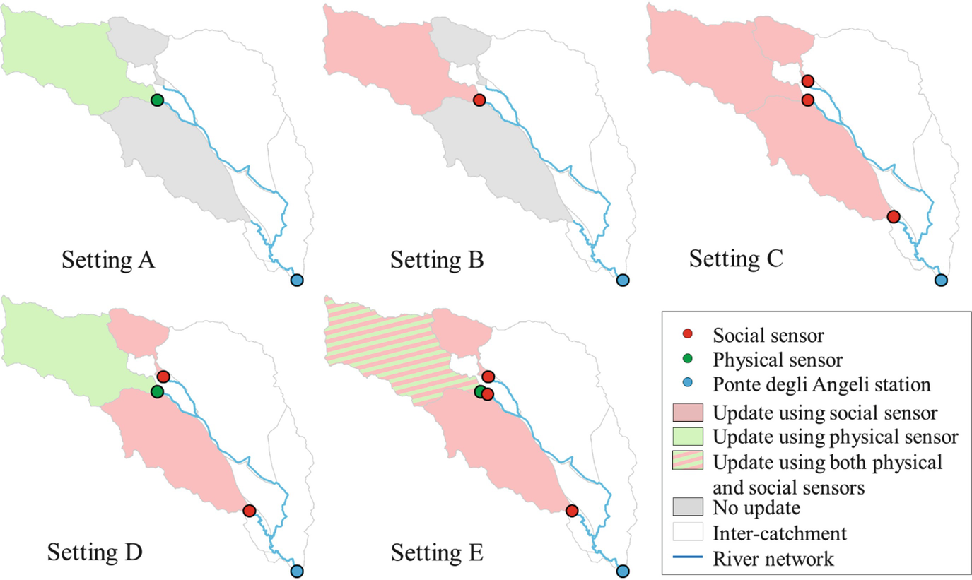
In the following, the contribution of assimilating synthetic flow data from a heterogeneous network of physical and social sensors on the semi-distributed model implemented in the Bacchiglione catchment is analysed. Streamflow observations from physical sensors are assumed to be synchronous with hourly frequency, while social observations are considered asynchronous with higher and irregular frequency. Five different experimental settings are introduced and represented in Fig. 9, corresponding to different types of sensors used.
Fig. 9
Different experimental settings implemented within the Bacchiglione catchment (based on [62])
The physical and social observations are assimilated in order to improve the poor model prediction at the catchment outlet (city of Vicenza) affected by an underestimation of the 3-day rainfall forecast used as normal input in flood forecasting practice in this area. Scenarios 10 and 11, described in Fig. 7, are used in this experiment in order to represent an irregular and random behaviour of the social observations.
Figure 10 shows the results obtained from the experiment settings represented in case of observations from distributed physical and social sensors. One of the main outcomes of these analyses is that the replacement of a physical sensor for a social sensor at only one location (settings B) does not improve the model performance in terms of NSE for different lead time values. Distributed locations of social sensors (setting C) can provide higher value of NSE than a single physical sensor, even for low number of observations in both regular and intermittent social observations. It is interesting to note that in case of integration between physical and social sensors (setting D), the NSE is higher than in case of setting C for low number of observations. However, with the higher number of observations, setting C is the one providing the best model improvement for low lead time values. Best model improvement is achieved in case of setting E. In case of intermittent observations (d, e and f), it can be noticed that the setting D provides higher improvement than setting C. In case of high lead time value (12 h), results of setting C tend to be similar to the ones obtained with setting B. As in case of scenario 10, also in case of scenario 11, the best results are achieved in case of setting E.
Fig. 10
Model performance expressed as μ(NSE) – assimilating different number of crowdsourced observations, for the three lead time values, having characteristic of scenario 10 (first row) and 11 (second row) (based on [63])
6 Conclusions
This chapter describes the novel methods mainly developed within the EU-FP7 WeSenseIt project, aimed to optimally assimilate heterogeneous intermittent observations, coming from static social sensors, to improve hydrological and hydrodynamic models for flood prediction. The proposed methods used to assimilate crowdsourced observations are applied to the Brue and Bacchiglione catchments, in which different hydrological and hydraulic models are implemented. A Kalman filter and ensemble Kalman filter are used to assimilate flow observations in linear and non-linear models, respectively. Observational error is assumed uniformly distributed with multiplying factors of 0.1 and 0.3 as minimum and maximum values for the static social sensors, respectively. It is worth noting that because real crowdsourced observations from citizen were not available at the time of this study, model-based synthetic realistic flow observations are used instead.
This study demonstrated that crowdsourced citizen-based observations can significantly improve flood prediction if integrated into hydrological and hydraulic models. In addition, networks of low-cost static and dynamic social sensors can actually complement traditional networks of static physical sensors, for the purpose of improving flood forecasting accuracy. This can be one of the potential applications of increasing efforts to build citizen observatories of water. On the one hand, citizens can play an active role in information capturing, evaluation and communication, and on the other hand, they can also help in improving models and increasing flood resilience.
In particular, assimilation of streamflow observations from static social sensors provides improvements in model performance which depends on the location of such observations and the structure of the considered hydrological model. Flood forecasts are influenced by the total number of social sensors and their locations in the case of semi-distributed model with sub-catchments connected in parallel, while results achieved with sub-catchment connected in series are more sensitive to the locations of the static physical sensors but not to their number.
This research proved that assimilation of asynchronous observations results in a significant improvement of NSE for different lead time values. Increasing the number of assimilated crowdsourced asynchronous observations within two model time steps induces an improvement in the NSE. However, after a threshold number of crowdsourced observations, NSE asymptotically approaches a certain value meaning that no improvement is achieved with additional observations.
Besides these important results, this work has still certain limitations which should be mentioned. Additional analyses on different case studies and hydrological/hydraulic model have to be carried out to draw more general conclusions about assimilation of the crowdsourced observations and their additional value in different types of catchments. In addition, the adopted simple hydrologic and flow propagation models neglect some of the physical processes in complex floodplains (e.g. lamination/reservoir effects). The internal states of the hydrologic model where crowdsourced observations are supposed to be observed should be calibrated, since unbiased models are necessary to optimise data assimilation frameworks [34]. Moreover, real-life crowdsourced observations provided by citizens using static social and dynamic social sensors have to be used to further validate the results obtained in this research.
Overall, with this research we demonstrated that the choice of the proper mathematical model and updating technique to be used for flood forecasting may vary according to the data availability, location of the sensors, type of forecast, etc.
Acknowledgements
This research was funded in the framework of the European FP7 Project WeSenseIt: Citizen Observatory of Water, grant agreement No. 308429.


 is the ensemble mean. The update states and Kalman gain are calculated using Eqs. (5) and (6). Because the EnKF performance is influenced by the spread of the ensemble [91–93], it is important to properly perturb the system in a way to obtain a reliable spread of the ensemble within a meaningful range [94]. For this reason, in this study we used the approach proposed by Anderson [91] to perturb the system and to evaluate the quality of the ensemble spread. More details are provided in Mazzoleni [63].