Earthquakes refer to any sudden shaking of the ground caused by the passage of seismic waves through Earth’s rocks. Seismic waves are produced when some form of energy stored in the Earth’s crust is suddenly released, usually when masses of rock straining against one another suddenly fracture and “slip.” Earthquakes occur most often along geologic faults, narrow zones where rock masses move in relation to one another. The major fault lines of the world are located at the fringes of the huge tectonic plates that make up Earth’s crust.
Little was understood about earthquakes until the emergence of seismology at the beginning of the 20th century. Seismology, which involves the scientific study of all aspects of earthquakes, has yielded answers to such long-standing questions as why and how earthquakes occur.
About 50,000 earthquakes large enough to be noticed without the aid of instruments occur annually over the entire Earth. Of these, approximately 100 are of sufficient size to produce substantial damage if their centres are near areas of habitation. Very great earthquakes occur on average about once per year. Over the centuries they have been responsible for millions of deaths and an incalculable amount of damage to property.
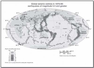
Distribution of seismic centres around the world where an earthquake with a magnitude of at least 5.5 occurred between 1975 and 1999. Encyclopædia Britannica, Inc.
Since earthquakes have the potential to cause extensive damage and great loss of life, scientists have long attempted to understand how they occur, their immediate and secondary effects, and the forces that govern how intense they are. The most common forces that spawn earthquakes are associated with plate movement and volcanism; however, they can be generated artificially. The strength felt from a given earthquake event depends largely on one’s distance away from the focus of the earthquake as well as the intensity of the seismic waves produced by the shifting rocks. Although damage often occurs in regions experiencing shaking ground, earthquakes can generate destructive tsunamis in the oceans that can affect areas thousands of miles away from the earthquake’s source.
Earth’s major earthquakes occur mainly in belts coinciding with the margins of tectonic plates. This has long been apparent from early catalogs of felt earthquakes and is even more readily discernible in modern seismicity maps, which show instrumentally determined epicentres. The most important earthquake belt is the Circum-Pacific Belt, which affects many populated coastal regions around the Pacific Ocean—for example, those of New Zealand, New Guinea, Japan, the Aleutian Islands, Alaska, and the western coasts of North and South America. It is estimated that 80 percent of the energy presently released in earthquakes comes from those whose epicentres are in this belt. The seismic activity is by no means uniform throughout the belt, and there are a number of branches at various points. Because at many places the Circum-Pacific Belt is associated with volcanic activity, it has been popularly dubbed the “Pacific Ring of Fire.”
A second belt, known as the Alpide Belt, passes through the Mediterranean region eastward through Asia and joins the Circum-Pacific Belt in the East Indies. The energy released in earthquakes from this belt is about 15 percent of the world total. There also are striking connected belts of seismic activity, mainly along oceanic ridges—including those in the Arctic Ocean, the Atlantic Ocean, and the western Indian Ocean—and along the rift valleys of East Africa. This global seismicity distribution is best understood in terms of its plate tectonic setting.
Earthquakes are caused by the sudden release of energy within some limited region of the rocks of Earth. The energy can be released by elastic strain, gravity, chemical reactions, or even the motion of massive bodies. Of all these the release of elastic strain is the most important cause, because this form of energy is the only kind that can be stored in sufficient quantity in Earth to produce major disturbances. Earthquakes associated with this type of energy release are called tectonic earthquakes.
Tectonic earthquakes are explained by the so-called elastic rebound theory, formulated by the American geologist Harry Fielding Reid after the San Andreas Fault ruptured in 1906, generating the great San Francisco earthquake. According to the theory, a tectonic earthquake occurs when strains in rock masses have accumulated to a point where the resulting stresses exceed the strength of the rocks, and sudden fracturing results. The fractures propagate rapidly through the rock, usually tending in the same direction and sometimes extending many kilometres along a local zone of weakness. In 1906, for instance, the San Andreas Fault slipped along a plane 430 km (270 miles) long. Along this line the ground was displaced horizontally as much as 6 metres (20 feet).
As a fault rupture progresses along or up the fault, rock masses are flung in opposite directions and thus spring back to a position where there is less strain. At any one point this movement may take place not at once but rather in irregular steps; these sudden slowings and restartings give rise to the vibrations that propagate as seismic waves. Such irregular properties of fault rupture are now included in the modeling of earthquake sources, both physically and mathematically. Roughnesses along the fault are referred to as asperities, and places where the rupture slows or stops are said to be fault barriers. Fault rupture starts at the earthquake focus, a spot that in many cases is close to 5–15 km under the surface. The rupture propagates in one or both directions over the fault plane until stopped or slowed at a barrier. Sometimes, instead of being stopped at the barrier, the fault rupture recommences on the far side; at other times the stresses in the rocks break the barrier, and the rupture continues.
Earthquakes have different properties depending on the type of fault slip that causes them. The usual fault model has a “strike” (that is, the direction from north taken by a horizontal line in the fault plane) and a “dip” (the angle from the horizontal shown by the steepest slope in the fault). The lower wall of an inclined fault is called the footwall. Lying over the footwall is the hanging wall. When rock masses slip past each other parallel to the strike, the movement is known as strike-slip faulting. Movement parallel to the dip is called dip-slip faulting. Strike-slip faults are right lateral or left lateral, depending on whether the block on the opposite side of the fault from an observer has moved to the right or left. In dip-slip faults, if the hanging-wall block moves downward relative to the footwall block, it is called “normal” faulting; the opposite motion, with the hanging wall moving upward relative to the footwall, produces reverse or thrust faulting.
All known faults are assumed to have been the seat of one or more earthquakes in the past, though tectonic movements along faults are often slow, and most geologically ancient faults are now aseismic (that is, they no longer cause earthquakes). The actual faulting associated with an earthquake may be complex, and it is often not clear whether in a particular earthquake the total energy issues from a single fault plane.
Observed geologic faults sometimes show relative displacements on the order of hundreds of kilometres over geologic time, whereas the sudden slip offsets that produce seismic waves may range from only several centimetres to tens of metres. In the 1976 Tangshan earthquake, for example, a surface strike-slip of about one metre was observed along the causative fault east of Beijing, and in the 1999 Taiwan earthquake the Chelung-pu fault slipped up to eight metres vertically.
A separate type of earthquake is associated with volcanic activity and is called a volcanic earthquake. Yet it is likely that even in such cases the disturbance is the result of a sudden slip of rock masses adjacent to the volcano and the consequent release of elastic strain energy. The stored energy, however, may in part be of hydrodynamic origin due to heat provided by magma moving in reservoirs beneath the volcano or to the release of gas under pressure.
There is a clear correspondence between the geographic distribution of volcanoes and major earthquakes, particularly in the Circum-Pacific Belt and along oceanic ridges. Volcanic vents, however, are generally several hundred kilometres from the epicentres of most major shallow earthquakes, and many earthquake sources occur nowhere near active volcanoes. Even in cases where an earthquake’s focus occurs directly below structures marked by volcanic vents, there is probably no immediate causal connection between the two activities; most likely both are the result of the same tectonic processes.
Earthquakes are sometimes caused by human activities, including the injection of fluids into deep wells, the detonation of large underground nuclear explosions, the excavation of mines, and the filling of large reservoirs. In the case of deep mining, the removal of rock produces changes in the strain around the tunnels. Slip on adjacent, preexisting faults or outward shattering of rock into the new cavities may occur. In fluid injection, the slip is thought to be induced by premature release of elastic strain, as in the case of tectonic earthquakes, after fault surfaces are lubricated by the liquid. Large underground nuclear explosions have been known to produce slip on already strained faults in the vicinity of the test devices.
Of the various earthquake-causing activities cited above, the filling of large reservoirs is among the most important. More than 20 significant cases have been documented in which local seismicity has increased following the impounding of water behind high dams. Often, causality cannot be substantiated, because no data exists to allow comparison of earthquake occurrence before and after the reservoir was filled. Reservoir-induction effects are most marked for reservoirs exceeding 100 metres (330 feet) in depth and 1 cubic km (0.24 cubic mile) in volume. Three sites where such connections have very probably occurred are the Hoover Dam in the United States, the Aswan High Dam in Egypt, and the Kariba Dam on the border between Zimbabwe and Zambia. The most generally accepted explanation for earthquake occurrence in such cases assumes that rocks near the reservoir are already strained from regional tectonic forces to a point where nearby faults are almost ready to slip. Water in the reservoir adds a pressure perturbation that triggers the fault rupture. The pressure effect is perhaps enhanced by the fact that the rocks along the fault have lower strength because of increased water-pore pressure. These factors notwithstanding, the filling of most large reservoirs has not produced earthquakes large enough to be a hazard.
The specific seismic source mechanisms associated with reservoir induction have been established in a few cases. For the main shock at the Koyna Dam and Reservoir in India (1967), the evidence favours strike-slip faulting motion. At both the Kremasta Dam in Greece (1965) and the Kariba Dam in Zimbabwe-Zambia (1961), the generating mechanism was dip-slip on normal faults. By contrast, thrust mechanisms have been determined for sources of earthquakes at the lake behind Nurek Dam in Tajikistan. More than 1,800 earthquakes occurred during the first nine years after water was impounded in this 317-metre-deep reservoir in 1972, a rate amounting to four times the average number of shocks in the region prior to filling.
In 1958 representatives from several countries, including the United States and the Soviet Union, met to discuss the technical basis for a nuclear test-ban treaty. Among the matters considered was the feasibility of developing effective means with which to detect underground nuclear explosions and to distinguish them seismically from earthquakes. After that conference, much special research was directed to seismology, leading to major advances in seismic signal detection and analysis.
Recent seismological work on treaty verification has involved using high-resolution seismographs in a worldwide network, estimating the yield of explosions, studying wave attenuation in Earth, determining wave amplitude and frequency spectra discriminants, and applying seismic arrays. The findings of such research have shown that underground nuclear explosions, compared with natural earthquakes, usually generate seismic waves through the body of Earth that are of much larger amplitude than the surface waves. This telltale difference along with other types of seismic evidence suggest that an international monitoring network of 270 seismographic stations could detect and locate all seismic events over the globe of magnitude 4 and above (corresponding to an explosive yield of about 100 tons of TNT).
Earthquakes have varied effects, including changes in geologic features, damage to man-made structures, and impact on human and animal life. Most of these effects occur on solid ground, but, since most earthquake foci are actually located under the ocean bottom, severe effects are often observed along the margins of oceans.
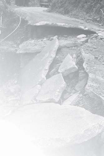
Earthquakes often cause dramatic geomorphological changes, including ground movements—either vertical or horizontal—along geologic fault traces; rising, dropping, and tilting of the ground surface; changes in the flow of groundwater; liquefaction of sandy ground; landslides; and mudflows. The investigation of topographic changes is aided by geodetic measurements, which are made systematically in a number of countries seriously affected by earthquakes.
Earthquakes can do significant damage to buildings, bridges, pipelines, railways, embankments, and other structures. The type and extent of damage inflicted are related to the strength of the ground motions and to the behaviour of the foundation soils. In the most intensely damaged region, called the meizoseismal area, the effects of a severe earthquake are usually complicated and depend on the topography and the nature of the surface materials. They are often more severe on soft alluvium and unconsolidated sediments than on hard rock. At distances of more than 100 km (60 miles) from the source, the main damage is caused by seismic waves traveling along the surface. In mines there is frequently little damage below depths of a few hundred metres even though the ground surface immediately above is considerably affected.
Earthquakes are frequently associated with reports of distinctive sounds and lights. The sounds are generally low-pitched and have been likened to the noise of an underground train passing through a station. The occurrence of such sounds is consistent with the passage of high-frequency seismic waves through the ground. Occasionally, luminous flashes, streamers, and bright balls have been reported in the night sky during earthquakes. These lights have been attributed to electric induction in the air along the earthquake source.
Following certain earthquakes, very long-wavelength water waves in oceans or seas sweep inshore. More properly called seismic sea waves or tsunamis (tsunami is a Japanese word for “harbour wave”), they are commonly referred to as tidal waves, although the attractions of the Moon and Sun play no role in their formation. They sometimes come ashore to great heights—tens of metres above mean tide level—and may be extremely destructive.
The usual immediate cause of a tsunami is sudden displacement in a seabed sufficient to cause the sudden raising or lowering of a large body of water. This deformation may be the fault source of an earthquake, or it may be a submarine landslide arising from an earthquake. Large volcanic eruptions along shorelines, such as those of Thera (c. 1580 BCE) and Krakatoa (1883 CE), have also produced notable tsunamis. The most destructive tsunami ever recorded occurred on Dec. 26, 2004, after an earthquake displaced the seabed off the coast of Sumatra, Indonesia. More than 200,000 people were killed by a series of waves that flooded coasts from Indonesia to Sri Lanka and even washed ashore on the Horn of Africa.
Following the initial disturbance to the sea surface, water waves spread in all directions. Their speed of travel in deep water is given by the formula (gh), where h is the sea depth and g is the acceleration of gravity. This speed may be considerable—100 metres per second (225 miles per hour) when h is 1,000 metres (3,300 feet). However, the amplitude (that is, the height of disturbance) at the water surface does not exceed a few metres in deep water, and the principal wavelength may be on the order of hundreds of kilometres; correspondingly, the principal wave period—that is, the time interval between arrival of successive crests—may be on the order of tens of minutes. Because of these features, tsunami waves are not noticed by ships far out at sea.
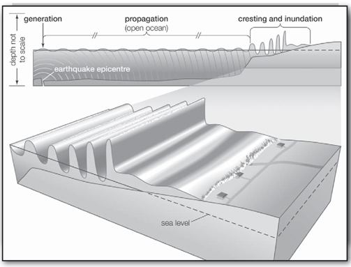
After being generated by an undersea earthquake or landslide, a tsunami may propagate unnoticed over vast reaches of open ocean before cresting in shallow water and inundating a coastline. Encyclopædia Britannica, Inc.
When tsunamis approach shallow water, however, the wave amplitude increases. The waves may occasionally reach a height of 20 to 30 metres above mean sea level in U- and V-shaped harbours and inlets. They characteristically do a great deal of damage in low-lying ground around such inlets. Frequently, the wave front in the inlet is nearly vertical, as in a tidal bore, and the speed of onrush may be on the order of 10 metres per second. In some cases there are several great waves separated by intervals of several minutes or more. The first of these waves is often preceded by an extraordinary recession of water from the shore, which may commence several minutes or even half an hour beforehand.
Organizations, notably in Japan, Siberia, Alaska, and Hawaii, have been set up to provide tsunami warnings. A key development is the Seismic Sea Wave Warning System, an internationally supported system designed to reduce loss of life in the Pacific Ocean. Centred in Honolulu, it issues alerts based on reports of earthquakes from circum-Pacific seismographic stations.
Seiches are rhythmic motions of water in nearly landlocked bays or lakes that are sometimes induced by earthquakes and tsunamis. Oscillations of this sort may last for hours or even for a day or two.
The great Lisbon earthquake of 1755 caused the waters of canals and lakes in regions as far away as Scotland and Sweden to go into observable oscillations. Seiche surges in lakes in Texas, in the southwestern United States, commenced between 30 and 40 minutes after the 1964 Alaska earthquake, produced by seismic surface waves passing through the area.
A related effect is the result of seismic waves from an earthquake passing through the seawater following their refraction through the seafloor. The speed of these waves is about 1.5 km (0.9 mile) per second, the speed of sound in water. If such waves meet a ship with sufficient intensity, they give the impression that the ship has struck a submerged object. This phenomenon is called a seaquake.
Earthquake intensity, or “strength,” and earthquake magnitude, or the “size” of the seismic waves, are distinct features of earthquakes that relate to the amount of energy released by the shifting rocks.
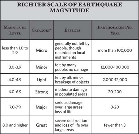
The violence of seismic shaking varies considerably over a single affected area. Because the entire range of observed effects is not capable of simple quantitative definition, the strength of the shaking is commonly estimated by reference to intensity scales that describe the effects in qualitative terms. Intensity scales date from the late 19th and early 20th centuries, before seismographs capable of accurate measurement of ground motion were developed. Since that time, the divisions in these scales have been associated with measurable accelerations of the local ground shaking. Intensity depends, however, in a complicated way not only on ground accelerations but also on the periods and other features of seismic waves, the distance of the measuring point from the source, and the local geologic structure. Furthermore, earthquake intensity, or strength, is distinct from earthquake magnitude, which is a measure of the amplitude, or size, of seismic waves as specified by a seismograph reading.
A number of different intensity scales have been set up during the past century and applied to both current and ancient destructive earthquakes. For many years the most widely used was a 10-point scale devised in 1878 by Michele Stefano de Rossi and François-Alphonse Forel. The scale now generally employed in North America is the Mercalli scale, as modified by Harry O. Wood and Frank Neumann in 1931, in which intensity is considered to be more suitably graded. A 12-point abridged form of the modified Mercalli scale is provided below. Modified Mercalli intensity VIII is roughly correlated with peak accelerations of about one-quarter that of gravity (g = 9.8 metres, or 32.2 feet, per second squared) and ground velocities of 20 cm (8 inches) per second. Alternative scales have been developed in both Japan and Europe for local conditions. The European (MSK) scale of 12 grades is similar to the abridged version of the Mercalli.
Earthquake magnitude is a measure of the “size,” or amplitude, of the seismic waves generated by an earthquake source and recorded by seismographs. (The types and nature of these waves are described in the section “Seismic Waves,” p. 247.) Because the size of earthquakes varies enormously, it is necessary for purposes of comparison to compress the range of wave amplitudes measured on seismograms by means of a mathematical device. In 1935 the American seismologist Charles F. Richter set up a magnitude scale of earthquakes as the logarithm to base 10 of the maximum seismic wave amplitude (in thousandths of a millimetre) recorded on a standard seismograph (the Wood-Anderson torsion pendulum seismograph) at a distance of 100 km (60 miles) from the earthquake epicentre. Reduction of amplitudes observed at various distances to the amplitudes expected at the standard distance of 100 km is made on the basis of empirical tables. Richter magnitudes ML are computed on the assumption that the ratio of the maximum wave amplitudes at two given distances is the same for all earthquakes and is independent of azimuth.
Richter first applied his magnitude scale to shallow-focus earthquakes recorded within 600 km of the epicentre in the southern California region. Later, additional empirical tables were set up, whereby observations made at distant stations and on seismographs other than the standard type could be used. Empirical tables were extended to cover earthquakes of all significant focal depths and to enable independent magnitude estimates to be made from body- and surface-wave observations.
At the present time a number of different magnitude scales are used by scientists and engineers as a measure of the relative size of an earthquake. The P-wave magnitude (Mb), for one, is defined in terms of the amplitude of the P wave recorded on a standard seismograph. Similarly, the surface-wave magnitude (Ms) is defined in terms of the logarithm of the maximum amplitude of ground motion for surface waves with a wave period of 20 seconds.
As defined, an earthquake magnitude scale has no lower or upper limit. Sensitive seismographs can record earthquakes with magnitudes of negative value and have recorded magnitudes up to about 9.0. (The 1906 San Francisco earthquake, for example, had a Richter magnitude of 8.25.)
A scientific weakness is that there is no direct mechanical basis for magnitude as defined above. Rather, it is an empirical parameter analogous to stellar magnitude assessed by astronomers. In modern practice a more soundly based mechanical measure of earthquake size is used—namely, the seismic moment (Mo). Such a parameter is related to the angular leverage of the forces that produce the slip on the causative fault. It can be calculated both from recorded seismic waves and from field measurements of the size of the fault rupture. Consequently, seismic moment provides a more uniform scale of earthquake size based on classical mechanics. This measure allows a more scientific magnitude to be used called moment magnitude (Mw). It is proportional to the logarithm of the seismic moment; values do not differ greatly from Ms values for moderate earthquakes. Given the above definitions, the great Alaska earthquake of 1964, with a Richter magnitude (ML) of 8.3, also had the values Ms = 8.4, M0 = 820 × 1027 dyne centimetres, and Mw = 9.2.
Energy in an earthquake passing a particular surface site can be calculated directly from the recordings of seismic ground motion, given, for example, as ground velocity. Such recordings indicate an energy rate of 105 watts per square metre (9,300 watts per square foot) near a moderate-size earthquake source. The total power output of a rupturing fault in a shallow earthquake is on the order of 1014 watts, compared with the 105 watts generated in rocket motors.
The surface-wave magnitude Ms has also been connected with the surface energy Es of an earthquake by empirical formulas. These give Es = 6.3 × 10¹¹ and 1.4 × 1025 ergs for earthquakes of Ms = 0 and 8.9, respectively. A unit increase in Ms corresponds to approximately a 32-fold increase in energy. Negative magnitudes Ms correspond to the smallest instrumentally recorded earthquakes, a magnitude of 1.5 to the smallest felt earthquakes, and one of 3.0 to any shock felt at a distance of up to 20 km (12 miles). Earthquakes of magnitude 5.0 cause light damage near the epicentre; those of 6.0 are destructive over a restricted area; and those of 7.5 are at the lower limit of major earthquakes.
The total annual energy released in all earthquakes is about 1025 ergs, corresponding to a rate of work between 10 million and 100 million kilowatts. This is approximately one one-thousandth the annual amount of heat escaping from Earth’s interior. Ninety percent of the total seismic energy comes from earthquakes of magnitude 7.0 and higher—that is, those whose energy is on the order of 1023 ergs or more.
There also are empirical relations for the frequencies of earthquakes of various magnitudes. Suppose N to be the average number of shocks per year for which the magnitude lies in a range about Ms. Then log10N = a − bMs fits the data well both globally and for particular regions; for example, for shallow earthquakes worldwide, a = 6.7 and b = 0.9 when Ms > 6.0. The frequency for larger earthquakes therefore increases by a factor of about 10 when the magnitude is diminished by one unit. The increase in frequency with reduction in Ms falls short, however, of matching the decrease in the energy E. Thus, larger earthquakes are overwhelmingly responsible for most of the total seismic energy release. The number of earthquakes per year with Mb > 4.0 reaches 50,000.
Earthquakes are the result of one plate, or portion of a plate, sliding against another. They may be preceded or followed by small shocks. Although the depth at which earthquake foci occurs can vary, most are considered shallow.
Global seismicity patterns had no strong theoretical explanation until the dynamic model called plate tectonics was developed during the late 1960s. This theory holds that Earth’s upper shell, or lithosphere, consists of nearly a dozen large, quasi-stable slabs called plates. The thickness of each of these plates is roughly 80 km (50 miles). The plates move horizontally relative to neighbouring plates at a rate of 1 to 10 cm (0.4 to 4 inches) per year over a shell of lesser strength called the asthenosphere. At the plate edges where there is contact between adjoining plates, boundary tectonic forces operate on the rocks, causing physical and chemical changes in them. New lithosphere is created at oceanic ridges by the upwelling and cooling of magma from Earth’s mantle. The horizontally moving plates are believed to be absorbed at the ocean trenches, where a subduction process carries the lithosphere downward into Earth’s interior. The total amount of lithospheric material destroyed at these subduction zones equals that generated at the ridges.
Seismological evidence (such as the location of major earthquake belts) is everywhere in agreement with this tectonic model. Earthquake sources are concentrated along the oceanic ridges, which correspond to divergent plate boundaries. At the subduction zones, which are associated with convergent plate boundaries, intermediate- and deep-focus earthquakes mark the location of the upper part of a dipping lithosphere slab. The focal mechanisms indicate that the stresses are aligned with the dip of the lithosphere underneath the adjacent continent or island arc.
Some earthquakes associated with oceanic ridges are confined to strike-slip faults, called transform faults, that offset the ridge crests. The majority of the earthquakes occurring along such horizontal shear faults are characterized by slip motions. Also in agreement with the plate tectonics theory is the high seismicity encountered along the edges of plates where they slide past each other. Plate boundaries of this kind, sometimes called fracture zones, include the San Andreas Fault in California and the North Anatolian fault system in Turkey. Such plate boundaries are the site of interplate earthquakes of shallow focus.
The low seismicity within plates is consistent with the plate tectonic description. Small to large earthquakes do occur in limited regions well within the boundaries of plates; however, such intraplate seismic events can be explained by tectonic mechanisms other than plate boundary motions and their associated phenomena.
Most parts of the world experience at least occasional shallow earthquakes—those that originate within 60 km (40 miles) of Earth’s outer surface. In fact, the great majority of earthquake foci are shallow. It should be noted, however, that the geographic distribution of smaller earthquakes is less completely determined than more severe quakes, partly because the availability of relevant data is dependent on the distribution of observatories.
Of the total energy released in earthquakes, 12 percent comes from intermediate earthquakes—that is, quakes with a focal depth ranging from about 60 to 300 km. About 3 percent of total energy comes from deeper earthquakes. The frequency of occurrence falls off rapidly with increasing focal depth in the intermediate range. Below intermediate depth the distribution is fairly uniform until the greatest focal depths, of about 700 km (430 miles), are approached.
The deeper-focus earthquakes commonly occur in patterns called Benioff zones that dip into Earth, indicating the presence of a subducting slab. Dip angles of these slabs average about 45°, with some shallower and others nearly vertical. Benioff zones coincide with tectonically active island arcs such as Japan, Vanuatu, Tonga, and the Aleutians, and they are normally but not always associated with deep ocean trenches such as those along the South American Andes. Exceptions to this rule include Romania and the Hindu Kush mountain system. In most Benioff zones, intermediate- and deep-earthquake foci lie in a narrow layer, although recent precise hypocentral locations in Japan and elsewhere show two distinct parallel bands of foci 20 km apart.
Usually, a major or even moderate earthquake of shallow focus is followed by many lesser-size earthquakes close to the original source region. This is to be expected if the fault rupture producing a major earthquake does not relieve all the accumulated strain energy at once. In fact, this dislocation is liable to cause an increase in the stress and strain at a number of places in the vicinity of the focal region, bringing crustal rocks at certain points close to the stress at which fracture occurs. In some cases an earthquake may be followed by 1,000 or more aftershocks a day.
Sometimes a large earthquake is followed by a similar one along the same fault source within an hour or perhaps a day. An extreme case of this is multiple earthquakes. In most instances, however, the first principal earthquake of a series is much more severe than the aftershocks. In general, the number of aftershocks per day decreases with time. The aftershock frequency is roughly inversely proportional to the time since the occurrence of the largest earthquake of the series.
Most major earthquakes occur without detectable warning, but some principal earthquakes are preceded by foreshocks. In another common pattern, large numbers of small earthquakes may occur in a region for months without a major earthquake. In the Matsushiro region of Japan, for instance, there occurred between August 1965 and August 1967 a series of hundreds of thousands of earthquakes, some sufficiently strong (up to Richter magnitude 5) to cause property damage but no casualties. The maximum frequency was 6,780 small earthquakes on April 17, 1966. Such series of earthquakes are called earthquake swarms. Earthquakes associated with volcanic activity often occur in swarms, though swarms also have been observed in many nonvolcanic regions.
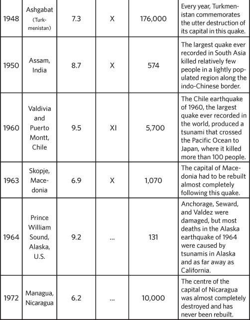
Earthquakes are among the most destructive natural events. On land, the upheaval caused by these phenomenon can cause landslides and collapse buildings, leading to tremendous numbers of human fatalities. In the oceans, the sudden movement of the seafloor rarely produces loss of life and property damage directly; however, tsunamis generated by such movement can promulgate across entire oceans to harm populations thousands of miles away. The following section details a number of earthquake events notable for the tolls they took on human lives.
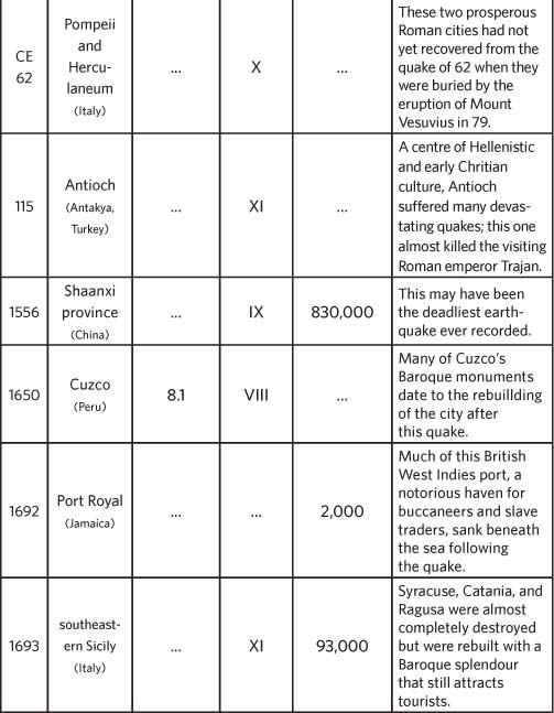
This earthquake, among the deadliest ever recorded, struck the Syrian city of Aleppo (Ḥalab) on Oct. 11, 1138. The city suffered extensive damage, and it is estimated that 230,000 people were killed.
Aleppo is located in northern Syria. The region, which sits on the boundary between the Arabian geologic plate and the African plate, is part of the Dead Sea Fault system. In the early 12th century this ancient Muslim city was home to tens of thousands of residents. On Oct. 10, 1138, a small shock shook the region, and some residents fled to surrounding towns. The main quake occurred the following day. As the city walls crumbled, rocks cascaded into the streets. Aleppo’s citadel collapsed, killing hundreds of residents.
Although Aleppo was the largest community affected by the earthquake, it likely did not suffer the worst of the damage. European Crusaders had constructed a citadel at nearby Ḥorim, which was leveled by the quake. A Muslim fort at Al-Atārib was destroyed as well, and several smaller towns and manned forts were reduced to rubble. The quake was allegedly felt as far away as Damascus, about 220 miles (350 km) to the south. The Aleppo earthquake was the first of several occurring between 1138 and 1139 that devastated areas in northern Syria and western Turkey.
On Jan. 23, 1556, a massive earthquake, believed to be the deadliest one ever recorded, occurred in Shaanxi province in northern China.
The earthquake (estimated at magnitude 8) struck Shaanxi and neighbouring Shanxi province to the east early on Jan. 23, 1556, killing or injuring an estimated 830,000 people. This massive death toll is thought to have reduced the population of the two provinces by about 60 percent. Local annals (which date to 1177 BCE) place the epicentre of the earthquake around Huaxian in Shaanxi. These annals, which record 26 other destructive earthquakes in the province, describe the destruction caused by the 1556 earthquake in a level of vivid detail that is unique among these records. Though the quake lasted only seconds, it leveled mountains, altered the path of rivers, caused massive flooding, and ignited fires that burned for days.
The local records indicate that, in addition to inspiring searches for the causes of earthquakes, this particular quake led the people in the region affected to search for ways to minimize the damage caused by such disasters. Many of the casualties in the quake were people who had been crushed by falling buildings. Thus, in the aftermath of the 1556 quake, many of the stone buildings that had been leveled were replaced with buildings made of softer, more earthquake-resistant materials, such as bamboo and wood.
The 1556 Shaanxi earthquake is associated with three major faults, which form the boundaries of the Wei River basin. All 26 of the earthquakes recorded in the annals had epicentres in this basin.
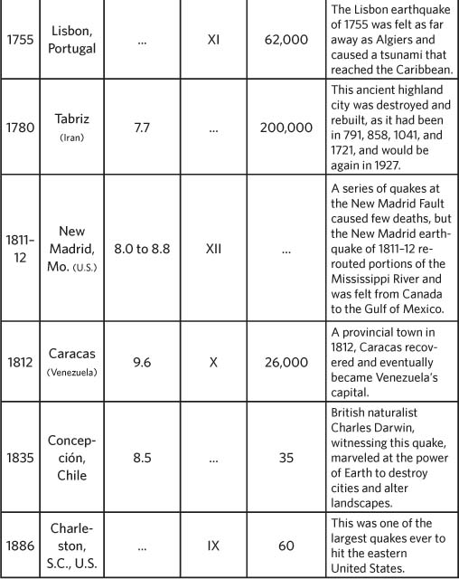
A series of earthquakes shook the port city of Lisbon, Port., on the morning of Nov. 1, 1755, causing serious damage and killing an estimated 60,000 people in Lisbon alone. Violent shaking demolished large public buildings and about 12,000 dwellings. Because November 1 is All Saints’ Day, a large part of the population was attending mass at the moment the earthquake struck; the churches, unable to withstand the seismic shock, collapsed, killing or injuring thousands of worshippers.
Modern research indicates that the main seismic source was faulting of the seafloor along the tectonic plate boundaries of the mid-Atlantic. The earthquake generated a tsunami that produced waves about 20 feet (6 metres) high at Lisbon and 65 feet (20 metres) high at Cádiz, Spain. The waves traveled westward to Martinique in the Caribbean Sea, a distance of 3,790 miles (6,100 km), in 10 hours and there reached a height of 13 feet (4 metres) above mean sea level. Damage was even reported in Algiers, 685 miles (1,100 km) to the east. The total number of persons killed included those who perished by drowning and in fires that burned throughout Lisbon for about six days following the shock. Depictions of the earthquakes in art and literature continued for centuries, making the “Great Lisbon Earthquake,” as it came to be known, a seminal event in European history.
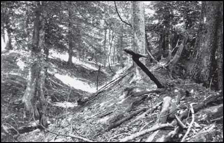
A series of three large earthquakes occurred near New Madrid in southern Missouri on Dec. 16, 1811 (magnitude from 8.0 to 8.5), and on Jan. 23 (magnitude 8.4) and Feb. 7, 1812 (magnitude 8.8). There were numerous aftershocks, of which 1,874 were large enough to be felt in Louisville, Ky., about 180 miles (300 km) away. The principal shock produced seismic waves of sufficient amplitude to shake down chimneys in Cincinnati, Ohio, about 360 miles (600 km) away. The waves were felt as far away as Canada in the north and the Gulf Coast in the south. The area of significant shaking was about 38,600 square miles (100,000 square km), considerably greater than the area involved in the San Francisco earthquake of 1906. Subsequently it was discovered that North American continental earthquakes, such as the Missouri shocks, produce greater shaking than do comparable shocks along the Pacific coast. In one region roughly 150 miles long by 37 miles wide (240 km by 60 km), the ground sank 3 to 9 feet (1 to 3 metres) and was covered by inflowing river water. In certain locations, forests were overthrown or ruined by the loss of soil shaken from the roots of the trees.
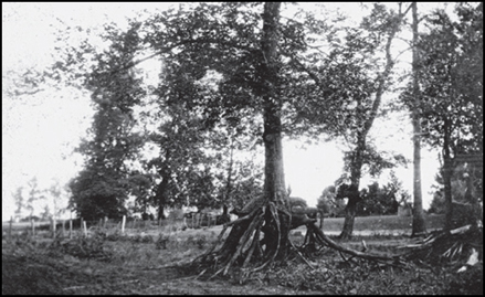
TOP: Tree with a double set of roots, formed in the aftermath of the New Madrid earthquakes (1811–12). The ground sank by several feet, creating low areas that were flooded by the Mississippi River. U.S. Geological Survey
BOTTOM: Landslide trench and ridge in the Chickasaw Bluffs east of Reelfoot Lake, Tenn., resulting from the New Madrid earthquakes (1811–12). U.S. Geological Survey
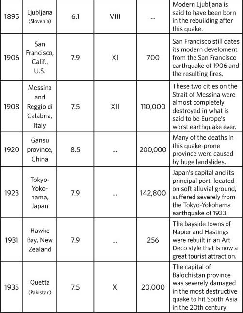
An earthquake and subsequent tsunami devastated southern Italy on Dec. 28, 1908. The double catastrophe almost completely destroyed Messina, Reggio di Calabria, and dozens of nearby coastal towns.
What was likely the most powerful recorded earthquake to hit Europe began at about 5:20 AM local time. Its epicentre was under the Strait of Messina, which separates the island of Sicily from the province of Calabria, the “toe” of Italy’s geographical “boot.” The main shock lasted for more than 20 seconds, and its magnitude reached 7.5 on the Richter scale. The tsunami that followed brought waves estimated to be 40 feet (13 metres) high crashing down on the coasts of northern Sicily and southern Calabria. More than 80,000 people were killed in the disaster. Many of the survivors were relocated to other Italian cities; others emigrated to the United States.
Experts long surmised that the tsunami resulted from seafloor displacement caused by the earthquake. However, research completed in the early 21st century suggested that an underwater landslide, unrelated to the earthquake, triggered the ensuing tsunami.
This earthquake, also called the Great Kanto earthquake, with a magnitude of 7.9 devastated the Tokyo-Yokohama metropolitan area near noon on Sept. 1, 1923. The death toll from this shock was estimated at more than 140,000.
A major earthquake with a magnitude of 7.9 occurred on April 18, 1906, at 5:12 AM off the northern California coast. The San Andreas Fault slipped along a segment about 270 miles (430 km) long, extending from San Juan Bautista in San Benito county to Humboldt county, and from there perhaps out under the sea to an unknown distance. The shaking was felt from Los Angeles in the south to Coos Bay, Oregon, in the north. Damage was severe in San Francisco and in other towns situated near the fault, including San Jose, Salinas, and Santa Rosa. At least 700 people were killed. In San Francisco the earthquake started a fire that destroyed the central business district. Geologic field studies of this earthquake led to the detailed formation of the theory that elastic rebound of strained faults causes the shaking associated with earthquakes. More than half of the brick buildings and one-tenth of the reinforced concrete structures collapsed. Many hundreds of thousands of houses were either shaken down or burned. The shock started a tsunami that reached a height of 39.5 feet (12 metres) at Atami on Sagami Gulf, where it destroyed 155 houses and killed 60 persons. The only comparable Japanese earthquake in the 20th century was at Kōbe on Jan. 16, 1995; about 5,500 people died amid considerable damage, which included widespread fires in the city and a landslide in nearby Nishinomiya.
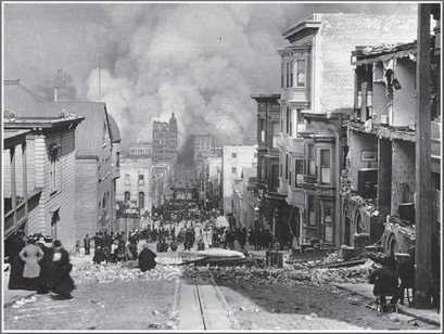
Crowds watching the fires set off by the earthquake in San Francisco in 1906. Photo by Arnold Genthe. Library of Congress, Washington, D.C.
This earthquake originated off the coast of Chile on May 22, 1960, with a moment magnitude of 9.5. The fault-displacement source of this earthquake, the largest in the world in the 20th century, extended over a distance of about 680 miles (1,100 km) along the southern Chilean coast. The cause was major underthrusting of the Pacific Plate under South America. Casualties included about 5,700 killed and 3,000 injured, and property damage in southern Chile amounted to roughly $550 million. Tsunamis triggered by the faulting caused human fatalities and property destruction in Hawaii, Japan, and the West Coast of the United States.
An earthquake that occurred in south-central Alaska on March 27, 1964, with a Richter scale magnitude of 9.2, this event released at least twice as much energy as the San Francisco earthquake of 1906 and was felt on land over an area of almost 502,000 square miles (1,300,000 square km). The death toll was only 131 because of the low density of the state’s population, but property damage was high. The earthquake tilted an area of at least 46,442 square miles (120,000 square km). Landmasses were thrust up locally as high as 82 feet (25 metres) to the east of a line extending northeastward from Kodiak Island through the western part of Prince William Sound. To the west, land sank as much as 8 feet (2.5 metres). Extensive damage in coastal areas resulted from submarine landslides and tsunamis. Tsunami damage occurred as far away as Crescent City, Calif. The occurrence of tens of thousands of aftershocks indicates that the region of faulting extended about 620 miles (1,000 km) along the North Pacific Plate subduction zone.
This earthquake, also called the Great Peruvian earthquake, originated off the coast of Peru on May 31, 1970, and caused massive landslides. More than 65,000 people died.
The epicentre of the earthquake was under the Pacific Ocean, about 15 miles (25 km) west of the Peruvian fishing port of Chimbote, in the Ancash department of north-central Peru. It occurred at about 3:20 PM local time and had a moment magnitude of 7.9. The effects of the quake could be felt from the northern city of Chiclayo south to the capital city of Lima, a distance of more than 400 miles (650 km). The most damage occurred in the coastal towns near the epicentre and in the Santa River valley. The destruction was exacerbated by the construction techniques used in the area; many homes and buildings were constructed using adobe, with many built on unstable soil.
Tens of thousands of people were killed or injured when their homes or businesses collapsed, and a significant number of victims died as the result of landslides triggered by the quake. The most destructive landslide fell from Peru’s highest mountain, Mount Huascarán, located in the west-central Andes. Fast-moving snow and earth swallowed the village of Yungay, buried much of Ranrahirca, and devastated other villages in the area.
Striking on July 28, 1976, with a magnitude of 8.0, this earthquake nearly razed the Chinese coal-mining and industrial city of Tangshan, located about 68 miles (110 km) east of Beijing. The death toll, thought to be one of the largest in recorded history, was officially reported as 242,000 persons, but it may have been as high as 655,000. At least 700,000 more people were injured, and property damage was extensive, reaching even to Beijing. Most of the fatalities resulted from the collapse of unreinforced masonry homes where people were sleeping.
The Mexico City earthquake possessed a moment magnitude of 8.0 whose main shock occurred at 7:18 AM on Sept. 19, 1985. The cause was a fault slip along the subduction slab under the Pacific coast of Mexico. Although 250 miles (400 km) from the epicentre, Mexico City suffered major building damage, and more than 10,000 of its inhabitants were reported killed. The highest intensity was in the central city, which is constructed on a former lake bed. The ground motion there measured five times that in the outlying districts, which have different soil foundations.
This major earthquake, also called the Loma Prieta earthquake, shook the San Francisco Bay Area, California, U.S., on Oct. 17, 1989. The strongest earthquake to hit the area since the San Francisco earthquake of 1906, it caused more than 60 deaths, thousands of injuries, and widespread property damage.
The earthquake was triggered by a slip along the San Andreas Fault. Its epicentre was in the Forest of Nisene Marks State Park, near Loma Prieta peak in the Santa Cruz mountains, northeast of Santa Cruz and approximately 60 miles (100 km) south of San Francisco. It began just after 5:00 PM local time and lasted approximately 15 seconds, with a magnitude of 7.1. The most severe damage was suffered by San Francisco and Oakland, but communities throughout the region, including Alameda, Santa Clara, Santa Cruz, and Monterey, also were affected. San Francisco’s Marina district was particularly hard hit because it had been built on filled land (comprising loose, sandy soil), and the unreinforced masonry buildings in Santa Cruz (many of which were 50 to 100 years old) failed spectacularly.
The earthquake significantly damaged the transportation system of the Bay Area. The collapse of the Cypress Street Viaduct (Nimitz Freeway) caused most of the earthquake-related deaths. The San Francisco–Oakland Bay Bridge was also damaged when a span of the top deck collapsed. In the aftermath, all bridges in the area underwent seismic retrofitting to make them more resistant to earthquakes.
Remarkably, the earthquake struck just before the start of the third game of the 1989 World Series, which was being played in San Francisco’s Candlestick Park between two Bay Area baseball teams, the San Francisco Giants and the Oakland Athletics. The disaster’s occurrence during a major live television broadcast meant that news of the earthquake, as well as aerial views provided by the Goodyear blimp, reached a large audience. The baseball championship, which was suspended for 10 days, would come to be known as the “Earthquake Series.”
The Northridge earthquake occurred in the densely populated San Fernando Valley in southern California, U.S., on Jan. 17, 1994. The third major earthquake to occur in the state in 23 years (after the 1971 San Fernando Valley and 1989 San Francisco–Oakland earthquakes), the Northridge earthquake was the state’s most destructive one since the San Francisco earthquake of 1906 and the costliest one in U.S. history.
The earthquake occurred just after 4:30 AM local time along a previously undiscovered blind thrust fault in the San Fernando Valley. Its epicentre was in Northridge, a suburb located about 20 miles (32 km) west-northwest of downtown Los Angeles. The major shock lasted 10–20 seconds and registered a magnitude of 6.7.
Fatality estimates range from just under 60 to more than 70 people killed, with most studies placing the number at around 60. The timing of the earthquake (early morning during a federal holiday) is thought to have prevented a higher death toll, as most residents were in their beds, rather than on failed freeways or in other collapsed structures (such as office buildings or parking lots). Most of the casualties occurred in wood-frame apartment buildings, popular in the San Fernando Valley, and particularly in those with weak first floors or lower-level parking garages.
Property damage was severe and widespread; although the worst damage was sustained by communities in the western and northern San Fernando Valley, other areas of Los Angeles county were affected, as were parts of Ventura, Orange, and San Bernardino counties. The percentage of buildings completely destroyed was relatively low in light of the strength of the ground motions. Nevertheless, tens of thousands of buildings were damaged, with many “red-tagged” as unsafe to enter and many more restricted to limited entry (“yellow-tagged”). A significant portion of the transportation system around Los Angeles was shut down, as sections of major freeways (including the Santa Monica Freeway and the Golden State Freeway) collapsed and numerous bridges sustained heavy damage. Fires that broke out in the San Fernando Valley and in Venice and Malibu caused additional harm.
The extent of the property damage in an area so well-prepared for earthquakes was staggering. Accordingly, a number of legislative changes were made in the aftermath of the Northridge earthquake. Most significantly, the state created the California Earthquake Authority, a publicly managed but privately funded organization offering basic residential earthquake insurance.
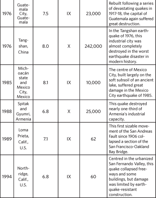
The large-scale Kōbe earthquake (Japanese: Hanshin-Awaji Daishinsai; “Great Hanshin-Awaji Earthquake Disaster”) shook the Ōsaka-Kōbe (Hanshin) metropolitan area of western Japan; it was among the strongest, deadliest, and costliest to ever strike that country.
The earthquake, also called the Great Hanshin earthquake, hit at 5:46 AM on Tuesday, Jan. 17, 1995, in the southern part of Hyogo prefecture, west-central Honshu. It lasted about 20 seconds and registered as a magnitude 6.9 (7.3 on the Richter scale). Its epicentre was the northern part of Awaji Island in the Inland Sea, 12.5 miles (20 km) off the coast of the port city of Kōbe; the quake’s focus was about 10 miles (16 km) below the earth’s surface. The Hanshin region (the name is derived from the characters used to write Ōsaka and Kōbe) is Japan’s second largest urban area, with more than 11 million inhabitants; with the earthquake’s epicentre located as close as it was to such a densely populated area, the effects were overwhelming. Its estimated death toll of 6,400 made it the worst earthquake to hit Japan since the Tokyo-Yokohama (Great Kant) earthquake of 1923, which had killed more than 140,000. The Kōbe quake’s devastation included 40,000 injured, more than 300,000 homeless residents, and in excess of 240,000 damaged homes, with millions of homes in the region losing electric or water service. Kōbe was the hardest hit city with 4,571 fatalities, more than 14,000 injured, and more than 120,000 damaged structures, more than half of which were fully collapsed. Portions of the Hanshin Expressway linking Kōbe and Ōsaka also collapsed or were heavily damaged during the earthquake.
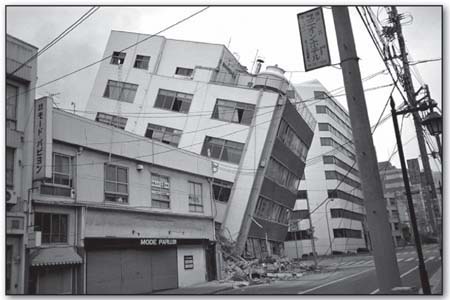
Building knocked off its foundation by the January 1995 earthquake in Kōbe, Japan. Dr. Roger Hutchison/NGDC
The earthquake was notable for exposing the vulnerability of the infrastructure. Authorities who had proclaimed the superior earthquake-resistance capabilities of Japanese construction were quickly proved wrong by the collapse of numerous supposedly earth-quake-resistant buildings, rail lines, elevated highways, and port facilities in the Kōbe area. Although most of the buildings that had been constructed according to new building codes withstood the earthquake, many others, particularly older wood-frame houses, did not. The transportation network was completely paralyzed, and the inadequacy of national disaster preparedness was also exposed. The government was heavily criticized for its slow and ineffectual response, as well as its initial refusal to accept help from foreign countries.
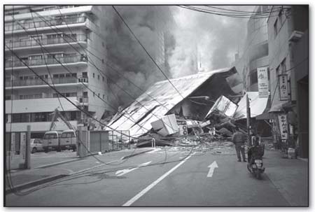
Burning and collapsed buildings in Kōbe, Japan, after the January 1995 earthquake. Dr. Roger Hutchison/NGDC
In the aftermath of the Kōbe disaster, roads, bridges, and buildings were reinforced against another earthquake, and the national government revised its disaster response policies (its response to the 2004 quake in Niigata prefecture was much faster and more effective). An emergency transportation network was also devised, and evacuation centres and shelters were set up in Kōbe by the Hyogo prefectural government.
Also referred to as the Kocaeli or the Gölcük earthquake, this devastating event, centred near the city of İzmit in northwestern Turkey, occurred on Aug. 17, 1999. Thousands of people were killed, and large parts of a number of mid-sized towns and cities were destroyed.
The earthquake, which occurred on the northernmost strand of the North Anatolian fault system, struck just after 3:00 AM local time. Its epicentre was about 7 miles (11 km) southeast of İzmit. The initial shock lasted less than a minute and registered a magnitude of 7.6. It was followed by two moderate aftershocks on August 19, about 50 miles (80 km) west of the original epicentre. More than 17,000 people were killed and an estimated 500,000 left homeless as thousands of buildings—chief among them the Turkish navy headquarters in Gölcük and the Tüpra![]() oil refinery in İzmit—collapsed or were heavily damaged. High casualty figures were reported in the towns of Gölcük, Derince, Darıca, and Sakarya (Adapazarı). Farther west, in Istanbul, the earthquake caused hundreds of fatalities and widespread destruction.
oil refinery in İzmit—collapsed or were heavily damaged. High casualty figures were reported in the towns of Gölcük, Derince, Darıca, and Sakarya (Adapazarı). Farther west, in Istanbul, the earthquake caused hundreds of fatalities and widespread destruction.
The rescue and relief effort was spearheaded by the Turkish Red Crescent and the Turkish army, with many international aid agencies joining in. The immediate support offered by Greece led to a thaw in the often-contentious relationship between the two neighbouring countries. Because most of the casualties resulted from the collapse of residential buildings, there was a strong public outcry against private contractors, who were accused of poor workmanship and of using cheap, inadequate materials. Some contractors were criminally prosecuted, but very few were found guilty. Public opinion also condemned officials who had failed to enforce building codes regarding earthquake-resistant designs.
This earthquake began at 1:47 AM local time on Sept. 21, 1999, below an epicentre 93 miles (150 km) south of Taipei, Taiwan. The death toll was 2,400 and some 10,000 people were injured. Thousands of houses collapsed, making more than 100,000 people homeless. The magnitude of the main shock was 7.7, resulting in about 10,000 buildings irreparably damaged and 7,500 partially damaged.
The earthquake, also called the 1999 Chi Chi earthquake, was produced by thrust faulting along the Chelung-pu fault in central Taiwan. The hanging wall thrust westward and upward along a line almost 60 miles (100 km) long, with uplift ranging from more than 3 feet (1 metre) in the south to 26 feet (8 metres) in the north. Many roads and bridges were damaged at their intersections with the fault displacement. The earthquake provided a wealth of observations for seismological research and engineering design; it is considered preeminent in the recording of strong ground shaking and crustal movement in the era of modern digital seismographs.
The Bhuj earthquake was a massive event that occurred on Jan. 26, 2001, in the Indian state of Gujarat, on the Pakistani border.
The earthquake struck near the town of Bhuj on the morning of India’s annual Republic Day (celebrating the creation of the Republic of India in 1950), and it was felt throughout much of northwestern India and parts of Pakistan. The moment magnitude of the quake was 7.7 (6.9 on the Richter scale). In addition to killing more than 20,000 people and injuring more than 150,000 others, the quake left hundreds of thousands homeless and destroyed or damaged more than a million buildings. A large majority of the local crops were ruined as well. Many people were still living in makeshift shelters a year later.
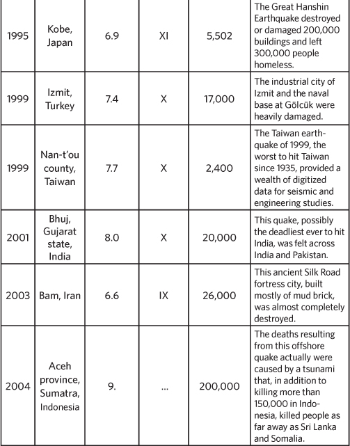
A disastrous earthquake centred in the Pakistan-administered portion of the Kashmir region and the North-West Frontier Province (NWFP) of Pakistan, the Kashmir earthquake also affected adjacent parts of India and Afghanistan. At least 79,000 people were killed and more than 32,000 buildings collapsed in Kashmir, with additional fatalities and destruction reported in India and Afghanistan.
The devastating earthquake struck on Saturday, Oct. 8, 2005, at 8:50 AM local time (03:50 UTC), with its epicentre approximately 65 miles (105 km) north-northeast of Islamabad, the capital of Pakistan. Measured at a magnitude of 7.6 (slightly less than that of the 1906 San Francisco quake), the earthquake caused major destruction in northern Pakistan, northern India, and Afghanistan, an area that lies on an active fault caused by the northward tectonic drift of the Indian subcontinent. The tremors were felt at a distance of up to 620 miles (1,000 km), as far away as Delhi and Punjab in northern India. The property loss caused by the quake left an estimated four million area residents homeless. The severity of the damage and the high number of fatalities were exacerbated by poor construction in the affected areas.
On May 12, 2008, a magnitude-7.9 earthquake brought enormous devastation to the mountainous central region of Sichuan province in southwestern China. The epicentre was in the city of Wenchuan, and some 80 percent of the structures in the area were flattened. Whole villages and towns in the mountains were destroyed, and many schools collapsed. China’s government quickly deployed 130,000 soldiers and other relief workers to the stricken area, but the damage from the earthquake made many remote villages difficult to reach, and the lack of modern rescue equipment caused delays that might have contributed to the number of deaths. In the aftermath, millions of people were left homeless, and some 90,000 were counted as dead or missing in the final assessment. Hundreds of dams, including two major ones, were found to have sustained damage. Some 200 relief workers were reported to have died in mud slides in the affected area, where damming of rivers and lakes by rocks, mud, and earthquake debris made flooding a major threat.
This large-scale earthquake occurred Jan. 12, 2010, at 4:53 PM, some 15 miles (24 km) southwest of the Haitian capital of Port-au-Prince. The initial shock registered a magnitude of 7.0 and was soon followed by two aftershocks of magnitudes 5.9 and 5.5. More aftershocks occurred in the following days, including another one of magnitude 5.9 that struck on January 20. Seismologists asserted that minor tremors would likely persist for months or even years. Haiti had not been hit by an earthquake of such enormity since the 18th century.
The earthquake was generated by the movement of the Caribbean tectonic plate eastward along the Enriquillo–Plantain Garden strike-slip fault system, a transform boundary that separates the Gonâve microplate—the fragment of the North American Plate upon which Haiti is situated—from the Caribbean Plate. Occurring at a depth of 8.1 miles (13 km), the temblor was fairly shallow, which increased the degree of shaking at the Earth’s surface. The collapsed buildings defining the landscape of the disaster area came as a consequence of Haiti’s lack of building codes. Without adequate reinforcement, the buildings disintegrated under the force of the quake. It was estimated that some three million people were affected by the quake—nearly one-third of the country’s total population. Of these, up to one million were left homeless.
The scientific discipline that is concerned with the study of earthquakes and of the propagation of seismic waves within Earth is called seismology. A branch of geophysics, it has provided much information about the composition and state of the planet’s interior.
The goals of seismological investigations may be local or regional, as in the attempt to determine subsurface faults and other structures in petroleum or mineral exploration, or they may be of global significance, as in attempts to determine structural discontinuities in Earth’s interior, the geophysical characteristics of island arcs, oceanic trenches, or mid-oceanic ridges, or the elastic properties of Earth materials generally.
In recent years, attention has been devoted to earthquake prediction and, more successfully, to assessing seismic hazards at different geographic sites in an effort to reduce the risks of earthquakes. The physics of seismic fault sources have been better determined and modeled for computer analysis. Moreover, seismologists have studied quakes induced by human activities, such as impounding water behind high dams and detonating underground nuclear explosions. The objective of the latter research is to find ways of discriminating between explosions and natural earthquakes. In order to predict where and when earthquakes will occur, scientists must first develop an understanding of the seismic waves that move through Earth and traverse along its surface. The measurement of these phenomena by seismometers, seismographs, and other instruments near fault lines (both on land and at the bottom of the ocean) allows scientists to detect earthquake patterns and construct models of earthquake behaviour. Such models can help structural engineers design buildings better able to withstand the forces generated by earthquakes. These tools also allow scientists to predict more accurately the time, location, and strength of impending earthquakes to warn people in affected areas.
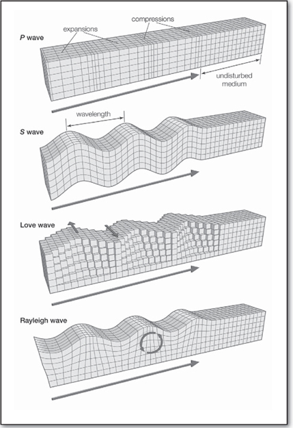
The vibration generated by an earthquake, explosion, or similar energetic source and propogated within Earth or along its surface is called a seismic wave. Earthquakes produce different types of seismic waves. Each type is classified according to the depth and medium in which it propagates.
Seismic waves generated by an earthquake source are commonly classified into four main types. The first two, the P (or primary) and S (or secondary) waves, propagate within the body of Earth, while the third and fourth, consisting of Love and Rayleigh waves, propagates along its surface. The existence of these types of seismic waves was mathematically predicted during the 19th century, and modern comparisons show that there is a close correspondence between such theoretical calculations and actual measurements of the seismic waves.
The P seismic waves travel as elastic motions at the highest speeds. They are longitudinal waves that can be transmitted by both solid and liquid materials in Earth’s interior. With P waves, the particles of the medium vibrate in a manner similar to sound waves—the transmitting media is alternately compressed and expanded. The slower type of body wave, the S wave, travels only through solid material. With S waves, the particle motion is transverse to the direction of travel and involves a shearing of the transmitting rock.
Because of their greater speed, P waves are the first to reach any point on Earth’s surface. The first P-wave onset starts from the spot where an earthquake originates. This point, usually at some depth within Earth, is called the focus, or hypocentre. The point at the surface immediately above the focus is known as the epicentre.
Of the two surface seismic waves, Love waves--named after the British seismologist A. E. H. Love, who first predicted their existence—travel faster. They follow along after the P and S waves have passed through the body of the planet. They are propagated when the solid medium near the surface has varying vertical elastic properties. Displacement of the medium by the wave is entirely perpendicular to the direction of propagation and has no vertical or longitudinal components. The energy of Love waves, like that of other surface waves, spreads from the source in two directions rather than in three, and so these waves produce a strong record at seismic stations even when originating from distant earthquakes.
The other principal surface waves are called Rayleigh waves after the British physicist Lord Rayleigh, who first mathematically demonstrated their existence. Both love and Rayleigh waves involve horizontal particle motion bu only the latter type has vertical ground displacements. Rayeigh waves travel along the free surface of an elastic solid such as Earth. Their motion is a combination of longitudinal compression and dilation that results in an elliptical motion of points on the surface. Of all seismic waves, Rayleigh waves spread out most in time, producing a long wave duration on seismographs. Even at substantial distances from the source inalluvial basins, Love and Rayleigh waves they cause much of the shaking felt during earthquakes.
At all distances from the focus, mechanical properties of the rocks, such as incompressibility, rigidity, and density, play a role in the speed with which the waves travel and the shape and duration of the wave trains. The layering of the rocks and the physical properties of surface soil also affect wave characteristics. In most cases, elastic behaviour occurs in earthquakes, but strong shaking of surface soils from the incident seismic waves sometimes results in nonelastic behaviour, including slumping (that is, the downward and outward movement of unconsolidated material) and the liquefaction of sandy soil.
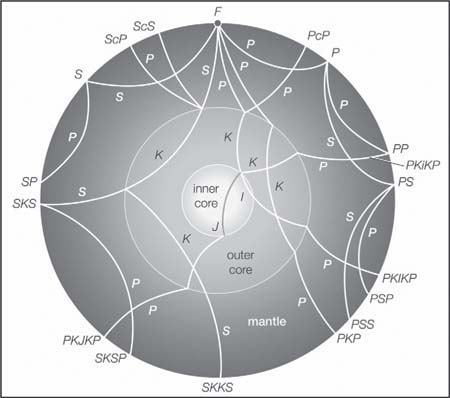
When a seismic wave encounters a boundary that separates rocks of different elastic properties, it undergoes reflection and refraction. There is a special complication because conversion between the wave types usually also occurs at such a boundary: an incident P or S wave can yield reflected P and S waves and refracted P and S waves. Boundaries between structural layers also give rise to diffracted and scattered waves. These additional waves are in part responsible for the complications observed in ground motion during earthquakes. Modern research is concerned with computing synthetic records of ground motion that are realistic in comparison with observed ground shaking, using the theory of waves in complex structures.
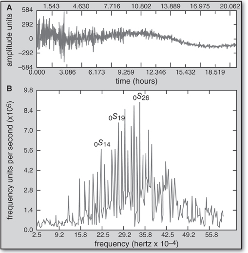
The frequency range of seismic waves is large, from as high as the audible range (greater than 20 hertz) to as low as the frequencies of the free oscillations of the whole Earth, with the gravest period being 54 minutes. Attenuation of the waves in rock imposes high-frequency limits, and in small to moderate earthquakes the dominant frequencies extend in surface waves from about 1 to 0.1 hertz.
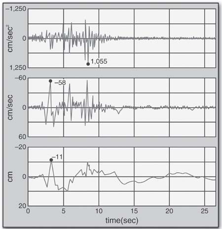
The amplitude range of seismic waves is also great in most earthquakes. Displacement of the ground ranges from 10−10 to 10−1 metre (4−12 to 4 inches). In the greatest earthquakes the ground amplitude of the predominant P waves may be several centimetres at periods of two to five seconds. Very close to the seismic sources of great earthquakes, investigators have measured large wave amplitudes with accelerations of the ground exceeding that of gravity (9.8 metres, or 32.2 feet, per second squared) at high frequencies and ground displacements of 1 metre at low frequencies.
The amplitude and frequency of seismic waves can be measured by a variety of instruments.
Seismographs are used to measure ground motion in both earthquakes and microseisms (small oscillations described below). Most of these instruments are of the pendulum type. Early mechanical seismographs had a pendulum of large mass (up to several tons) and produced seismograms by scratching a line on smoked paper on a rotating drum. In later instruments, seismograms were recorded by means of a ray of light from the mirror of a galvanometer through which passed an electric current generated by electromagnetic induction when the pendulum of the seismograph moved. Technological developments in electronics have given rise to higher-precision pendulum seismometers and sensors of ground motion. In these instruments the electric voltages produced by motions of the pendulum or the equivalent are passed through electronic circuitry to amplify and digitize the ground motion for more exact readings.
Generally speaking, seismographs are divided into three types: short-period, long- (or intermediate-) period, and ultralong-period, or broadband, instruments. Short-period instruments are used to record P and S body waves with high magnification of the ground motion. For this purpose, the seismograph response is shaped to peak at a period of about one second or less. The intermediate-period instruments of the type used by the World-Wide Standardized Seismographic Network (described in the section “Earthquake Observatories”) had a response maximum at about 20 seconds. Recently, in order to provide as much flexibility as possible for research work, the trend has been toward the operation of very broadband seismographs with digital representation of the signals. This is usually accomplished with very long-period pendulums and electronic amplifiers that pass signals in the band between 0.005 and 50 hertz.
When seismic waves close to their source are to be recorded, special design criteria are needed. Instrument sensitivity must ensure that the largest ground movements can be recorded without exceeding the upper scale limit of the device. For most seismological and engineering purposes the wave frequencies that must be recorded are higher than 1 hertz, and so the pendulum or its equivalent can be small. For this reason accelerometers that measure the rate at which the ground velocity is changing have an advantage for strong-motion recording. Integration is then performed to estimate ground velocity and displacement. The ground accelerations to be registered range up to two times that of gravity. Recording such accelerations can be accomplished mechanically with short torsion suspensions or force-balance mass-spring systems.
Because many strong-motion instruments need to be placed at unattended sites in ordinary buildings for periods of months or years before a strong earthquake occurs, they usually record only when a trigger mechanism is actuated with the onset of ground motion. Solid-state memories are now used, particularly with digital recording instruments, making it possible to preserve the first few seconds before the trigger starts the permanent recording and to store digitized signals on magnetic cassette tape or on a memory chip. In past design absolute timing was not provided on strong-motion records but only accurate relative time marks; the present trend, however, is to provide Universal Time (the local mean time of the prime meridian) by means of special radio receivers, small crystal clocks, or GPS (global positioning system) receivers from satellite clocks.
The prediction of strong ground motion and response of engineered structures in earthquakes depends critically on measurements of the spatial variability of earthquake intensities near the seismic wave source. In an effort to secure such measurements, special arrays of strong-motion seismographs have been installed in areas of high seismicity around the world. Large-aperture seismic arrays (linear dimensions on the order of 1 to 10 km, or 0.6 to 6 miles) of strong-motion accelerometers can now be used to improve estimations of speed, direction of propagation, and types of seismic wave components. Particularly important for full understanding of seismic wave patterns at the ground surface is measurement of the variation of wave motion with depth. To aid in this effort, special digitally recording seismometers have been installed in deep boreholes.
Because 70 percent of Earth’s surface is covered by water, there is a need for ocean-bottom seismometers to augment the global land-based system of recording stations. Field tests have established the feasibility of extensive long-term recording by instruments on the seafloor. Japan already has a semipermanent seismograph system of this type that was placed on the seafloor off the Pacific coast of central Honshu in 1978 by means of a cable.
Because of the mechanical difficulties of maintaining permanent ocean-bottom instrumentation, different systems have been considered. They all involve placement of instruments on the bottom of the ocean, though they employ various mechanisms for data transmission. Signals may be transmitted to the ocean surface for retransmission by auxiliary apparatus or transmitted via cable to a shore-based station. Another system is designed to release its recording device automatically, allowing it to float to the surface for later recovery.
The use of ocean-bottom seismographs should yield much-improved global coverage of seismic waves and provide new information on the seismicity of oceanic regions. Ocean-bottom seismographs will enable investigators to determine the details of the crustal structure of the seafloor and, because of the relative thinness of the oceanic crust, should make it possible to collect clear seismic information about the upper mantle. Such systems are also expected to provide new data on plate boundaries, on the origin and propagation of microseisms, and on the nature of ocean-continent margins.
Small ground motions known as microseisms are commonly recorded by seismographs. These weak wave motions are not generated by earthquakes, and they complicate accurate recording of the latter. However, they are of scientific interest because their form is related to the Earth’s surface structure.
Some microseisms have local causes—for example, those due to traffic or machinery or due to local wind effects, storms, and the action of rough surf against an extended steep coast. Another class of microseisms exhibits features that are very similar on records traced at earthquake observatories that are widely separated, including approximately simultaneous occurrence of maximum amplitudes and similar wave frequencies. These microseisms may persist for many hours and have more or less regular periods of about five to eight seconds. The largest amplitudes of such microseisms are on the order of 10−3 cm (0.0004 inch) and occur in coastal regions. The amplitudes also depend to some extent on local geologic structure. Some microseisms are produced when large standing water waves are formed far out at sea. The period of this type of microseism is half that of the standing wave.
Worldwide during the late 1950s, there were only about 700 seismographic stations, which were equipped with seismographs of various types and frequency responses. Few instruments were calibrated; actual ground motions could not be measured, and timing errors of several seconds were common. The World-Wide Standardized Seismographic Network (WWSSN), the first modern worldwide standardized system, was established to help remedy this situation. Each station of the WWSSN had six seismographs—three short-period and three long-period seismographs. Timing and accuracy were maintained by crystal clocks, and a calibration pulse was placed daily on each record. By 1967 the WWSSN consisted of about 120 stations distributed over 60 countries. The resulting data provided the basis for significant advances in research on earthquake mechanisms, global tectonics, and the structure of Earth’s interior.
By the 1980s a further upgrading of permanent seismographic stations began with the installation of digital equipment by a number of organizations. Among the global networks of digital seismographic stations now in operation are the Seismic Research Observatories in boreholes 100 metres (330 feet) deep and modified high-gain, long-period surface observatories. The Global Digital Seismographic Network in particular has remarkable capability, recording all motions from Earth tides to microscopic ground motions at the level of local ground noise. At present there are about 128 sites. With this system the long-term seismological goal will have been accomplished to equip global observatories with seismographs that can record every small earthquake anywhere over a broad band of frequencies.
Many observatories make provisional estimates of the epicentres of important earthquakes. These estimates provide preliminary information locally about particular earthquakes and serve as first approximations for the calculations subsequently made by large coordinating centres.
If an earthquake’s epicentre is less than 105° away from an observatory, the epicentre’s position can often be estimated from the readings of three seismograms recording perpendicular components of the ground motion. For a shallow earthquake the epicentral distance is indicated by the interval between the arrival times of P and S waves; the azimuth and angle of wave emergence at the surface are indicated by a comparison of the sizes and directions of the first movements shown in the seismograms and by the relative sizes of later waves, particularly surface waves. It should be noted, however, that in certain regions the first wave movement at a station arrives from a direction differing from the azimuth toward the epicentre. This anomaly is usually explained by strong variations in geologic structures.
When data from more than one observatory are available, an earthquake’s epicentre may be estimated from the times of travel of the P and S waves from source to recorder. In many seismically active regions, networks of seismographs with telemetry transmission and centralized timing and recording are common. Whether analog or digital recording is used, such integrated systems greatly simplify observatory work: multichannel signal displays make identification and timing of phase onsets easier and more reliable. Moreover, online microprocessors can be programmed to pick automatically, with some degree of confidence, the onset of a significant common phase, such as P, by correlation of waveforms from parallel network channels. With the aid of specially designed computer programs, seismologists can then locate distant earthquakes to within about 10 km (6 miles) and the epicentre of a local earthquake to within a few kilometres.
Catalogs of earthquakes felt by humans and of earthquake observations have appeared intermittently for many centuries. The earliest known list of instrumentally recorded earthquakes with computed times of origin and epicentres is for the period 1899–1903. In subsequent years, cataloging of earthquakes has become more uniform and complete. Especially valuable is the service provided by the International Seismological Centre (ISC) at Newbury, Eng. Each month it receives more than 1,000,000 readings from more than 2,000 stations worldwide and preliminary estimates of the locations of approximately 1,600 earthquakes from national and regional agencies and observatories. The ISC publishes a monthly bulletin—with about a two-year delay—that provides all available information on each of more than 5,000 earthquakes.
Various national and regional centres control networks of stations and act as intermediaries between individual stations and the international organizations. Examples of long-standing national centres include the Japan Meteorological Agency and United States National Earthquake Information Center in Colorado (a subdivision of the United States Geological Survey). These centres normally make estimates of the magnitudes, epicentres, origin times, and focal depths of local earthquakes. On the Internet, data on global seismicity is continually accessible through the Web site of the Incorporated Research Institutions for Seismology (IRIS).
An important research technique is to infer the character of faulting in an earthquake from the recorded seismograms. For example, observed distributions of the directions of the first onsets in waves arriving at the Earth’s surface have been effectively used. Onsets are called “compressional” or “dilatational” according to whether the direction is away from or toward the focus, respectively. A polarity pattern becomes recognizable when the directions of the P-wave onsets are plotted on a map—there are broad areas in which the first onsets are predominantly compressions, separated from predominantly dilatational areas by nodal curves near which the P-wave amplitudes are abnormally small.
In 1926 the American geophysicist Perry E. Byerly used patterns of P onsets over the entire globe to infer the orientation of the fault plane in a large earthquake. The polarity method yields two P-nodal curves at Earth’s surface; one curve is in the plane containing the assumed fault, and the other is in the plane (called the auxiliary plane) that passes through the focus and is perpendicular to the forces of the plane. The recent availability of worldwide broad-based digital recording has enabled computer programs to be written that estimate the fault mechanism and seismic moment from the complete pattern of seismic wave arrivals. Given a well-determined pattern at a number of earthquake observatories, it is possible to locate two planes, one of which is the plane containing the fault.
The search for periodic cycles in earthquake occurrence is an old one. Generally, periodicities in time and space for major earthquakes have not been widely detected or accepted. One problem is that long-term earthquake catalogs are not homogeneous in their selection and reporting. The most extensive catalog of this kind comes from China and begins about 700 BCE. The catalog contains some information on about 1,000 destructive earthquakes. The sizes of these earthquakes have been assessed from the reports of damage, intensity, and shaking.
Another approach to the statistical occurrence of earthquakes involves the postulation of trigger forces that initiate the rupture. Such forces have been attributed to severe weather conditions, volcanic activity, and tidal forces, for example. Usually correlations are made between the physical phenomena assumed to provide the trigger and the repetition of earthquakes. Inquiry must always be made to discover whether a causative link is actually present, but in no cases to the present has a trigger mechanism, at least for moderate to large earthquakes, been unequivocally found that satisfies the various necessary criteria.
Statistical methods also have been tried with populations of regional earthquakes. It has been suggested, but never established generally, that the slope b of the regression line between the logarithm of the number of earthquakes and the magnitude for a region may change characteristically with time. Specifically, the claim is that the b value for the population of foreshocks of a major earthquake may be significantly smaller than the mean b value for the region averaged over a long interval of time.
The elastic rebound theory of earthquake sources allows rough prediction of the occurrence of large shallow earthquakes. Harry F. Reid gave, for example, a crude forecast of the next great earthquake near San Francisco. (The theory also predicted, of course, that the place would be along the San Andreas or an associated fault.) The geodetic data indicated that during an interval of 50 years relative displacements of 3.2 metres (10.5 feet) had occurred at distant points across the fault. The maximum elastic-rebound offset along the fault in the 1906 earthquake was 6.5 metres. Therefore, (6.5 3.2) × 50, or about 100, years would again elapse before sufficient strain accumulated for the occurrence of an earthquake comparable to that of 1906. The premises are that the regional strain will grow uniformly and that various constraints have not been altered by the great 1906 rupture itself (such as by the onset of slow fault slip). Such strain rates are now being more adequately measured along a number of active faults such as the San Andreas, using networks of GPS sensors.
For many years prediction research has been influenced by the basic argument that strain accumulates in the rock masses in the vicinity of a fault and results in crustal deformation. Deformations have been measured in the horizontal direction along active faults (by trilateration and triangulation) and in the vertical direction by precise leveling and tiltmeters. Some investigators believe that changes in groundwater level occur prior to earthquakes; variations of this sort have been reported mainly from China. Because water levels in wells respond to a complex array of factors such as rainfall, such factors will have to be removed if changes in water level are to be studied in relation to earthquakes.
The theory of dilatancy (that is, an increase in volume) of rock prior to rupture once occupied a central position in discussions of premonitory phenomena of earthquakes, but it now receives less support. It is based on the observation that many solids exhibit dilatancy during deformation. For earthquake prediction the significance of dilatancy, if real, is in its effects on various measurable quantities of Earth’s crust, such as seismic velocities, electric resistivity, and ground and water levels. The best-studied consequence is the effect on seismic velocities. The influence of internal cracks and pores on the elastic properties of rocks can be clearly demonstrated in laboratory measurements of those properties as a function of hydrostatic pressure. In the case of saturated rocks, experiments predict—for shallow earthquakes—that dilatancy occurs as a portion of the crust is stressed to failure, causing a decrease in the velocities of seismic waves. Recovery of velocity is brought about by subsequent rise of the pore pressure of water, which also has the effect of weakening the rock and enhancing fault slip.
Strain buildup in the focal region may have measurable effects on other observable properties, including electrical conductivity and gas concentration. Because the electrical conductivity of rocks depends largely on interconnected water channels within the rocks, resistivity may increase before the cracks become saturated. As pore fluid is expelled from the closing cracks, the local water table would rise and concentrations of gases such as radioactive radon would increase. No unequivocal confirming measurements have yet been published.
Geologic methods of extending the seismicity record back from the present also are being explored. Field studies indicate that the sequence of surface ruptures along major active faults associated with large earthquakes can sometimes be constructed. An example is the series of large earthquakes in Turkey in the 20th century, which were caused mainly by successive westward ruptures of the North Anatolian Fault. Liquefaction effects preserved in beds of sand and peat have provided evidence—when radiometric dating methods are used—for large paleoearthquakes extending back for more than 1,000 years in many seismically active zones, including the Pacific Northwest coast of the United States.
Less well-grounded precursory phenomena, particularly earthquake lights and animal behaviour, sometimes draw more public attention than the precursors discussed above. Many reports of unusual lights in the sky and abnormal animal behaviour preceding earthquakes are known to seismologists, mostly in anecdotal form. Both these phenomena are usually explained in terms of a release of gases prior to earthquakes and electric and acoustic stimuli of various types. At present there is no definitive experimental evidence to support claims that animals sometimes sense the coming of an earthquake.
Considerable work has been done in seismology to explain the characteristics of the recorded ground motions in earthquakes. Such knowledge is needed to predict ground motions in future earthquakes so that earthquake-resistant structures can be designed. Although earthquakes cause death and destruction through such secondary effects as landslides, tsunamis, fires, and fault rupture, the greatest losses—both of lives and of property—result from the collapse of man-made structures during the violent shaking of the ground. Accordingly, the most effective way to mitigate the damage of earthquakes from an engineering standpoint is to design and construct structures capable of withstanding strong ground motions.
Most elastic waves recorded close to an extended fault source are complicated and difficult to interpret uniquely. Understanding such near-source motion can be viewed as a three-part problem. The first part stems from the generation of elastic waves by the slipping fault as the moving rupture sweeps out an area of slip along the fault plane within a given time. The pattern of waves produced is dependent on several parameters, such as fault dimension and rupture velocity. Elastic waves of various types radiate from the vicinity of the moving rupture in all directions. The geometry and frictional properties of the fault critically affect the pattern of radiation from it.
The second part of the problem concerns the passage of the waves through the intervening rocks to the site and the effect of geologic conditions. The third part involves the conditions at the recording site itself, such as topography and highly attenuating soils. All these questions must be considered when estimating likely earthquake effects at a site of any proposed structure.
Experience has shown that the ground strong-motion recordings have a variable pattern in detail but predictable regular shapes in general (except in the case of strong multiple earthquakes). In a strong horizontal shaking of the ground near the fault source, there is an initial segment of motion made up mainly of P waves, which frequently manifest themselves strongly in the vertical motion. This is followed by the onset of S waves, often associated with a longer-period pulse of ground velocity and displacement related to the near-site fault slip or fling. This pulse is often enhanced in the direction of the fault rupture and normal to it. After the S onset there is shaking that consists of a mixture of S and P waves, but the S motions become dominant as the duration increases. Later, in the horizontal component, surface waves dominate, mixed with some S body waves. Depending on the distance of the site from the fault and the structure of the intervening rocks and soils, surface waves are spread out into long trains.
Recording of the San Fernando earthquake, near Pacoima Dam, California, 1971, showing (top) ground acceleration, (centre) velocity, and (bottom) displacement. Encyclopædia Britannica, Inc.
In many regions, seismic expectancy maps or hazard maps are now available for planning purposes. The anticipated intensity of ground shaking is represented by a number called the peak acceleration or the peak velocity.
To avoid weaknesses found in earlier earthquake hazard maps, the following general principles are usually adopted today:
1. The map should take into account not only the size but also the frequency of earthquakes.
2. The broad regionalization pattern should use historical seismicity as a database, including the following factors: major tectonic trends, acceleration attenuation curves, and intensity reports.
3. Regionalization should be defined by means of contour lines with design parameters referred to ordered numbers on neighbouring contour lines (this procedure minimizes sensitivity concerning the exact location of boundary lines between separate zones).
4. The map should be simple and not attempt to microzone the region.
5. The mapped contoured surface should not contain discontinuities, so that the level of hazard progresses gradually and in order across any profile drawn on the map.
Developing engineered structural designs that are able to resist the forces generated by seismic waves can be achieved either by following building codes based on hazard maps or by appropriate methods of analysis. Many countries reserve theoretical structural analyses for the larger, more costly, or critical buildings to be constructed in the most seismically active regions, while simply requiring that ordinary structures conform to local building codes. Economic realities usually determine the goal, not of preventing all damage in all earthquakes but of minimizing damage in moderate, more common earthquakes and ensuring no major collapse at the strongest intensities. An essential part of what goes into engineering decisions on design and into the development and revision of earthquake-resistant design codes is therefore seismological, involving measurement of strong seismic waves, field studies of intensity and damage, and the probability of earthquake occurrence.
Earthquake risk can also be reduced by rapid post-earthquake response. Strong-motion accelerographs have been connected in some urban areas, such as Los Angeles, Tokyo, and Mexico City, to interactive computers. The recorded waves are correlated with seismic intensity scales and rapidly displayed graphically on regional maps via the World Wide Web.
Seismological data on Earth’s deep structure come from several sources. These include P and S waves in earthquakes and nuclear explosions, the dispersion of surface waves from distant earthquakes, and vibrations of the whole Earth from large earthquakes.
One of the major aims of seismology is to infer the minimum set of properties of Earth’s interior that will explain recorded seismic wave trains in detail. Notwithstanding the tremendous progress made in the exploration of Earth’s deep structure during the first half of the 20th century, realization of this goal was severely limited until the 1960s because of the laborious effort required to evaluate theoretical models and to process the large amounts of earthquake data recorded. The application of high-speed computers with their enormous storage and rapid retrieval capabilities opened the way for major advances in both theoretical work and data handling.
Since the mid-1970s, researchers have studied realistic models of Earth’s structure that include continental and oceanic boundaries, mountains, and river valleys rather than simple structures such as those involving variation only with depth. In addition, various technical developments have benefited observational seismology. For example, the implications of seismic exploratory techniques developed by the petroleum industry (such as seismic reflection) have been recognized and the procedures adopted. Equally significant has been the application of three-dimensional imaging methods to the exploration of Earth’s deep structure. This has been made possible by the development of very fast microprocessors and computers with peripheral display equipment.
The major method for determining the structure of Earth’s deep interior is the detailed analysis of seismograms of seismic waves. (Such earthquake readings also provide estimates of wave velocities, density, and elastic and inelastic parameters in Earth.) The primary procedure is to measure the travel times of various wave types, such as P and S, from their source to the recording seismograph. First, however, identification of each wave type with its ray path through Earth must be made.
Rays corresponding to waves that have been reflected at Earth’s outer surface (or possibly at one of the interior discontinuity surfaces) are denoted as PP, PS, SP, PSS, and so on. For example, P S corresponds to a wave that is of P type before surface reflection and of S type afterward. In addition, there are rays such as p P P, s P P, and s P S, the symbols p and s corresponding to an initial ascent to the outer surface as P or S waves, respectively, from a deep focus.
An especially important class of rays is associated with a discontinuity surface separating the central core of Earth from the mantle at a depth of about 2,900 km (1,800 miles) below the outer surface. The symbol c is used to indicate an upward reflection at this discontinuity. Thus, if a P wave travels down from a focus to the discontinuity surface in question, the upward reflection into an S wave is recorded at an observing station as the ray P c S and similarly with P c P, S c S, and S c P. The symbol K is used to denote the part (of P type) of the path of a wave that passes through the liquid central core. Thus, the ray S K S corresponds to a wave that starts as an S wave, is refracted into the central core as a P wave, and is refracted back into the mantle, wherein it finally emerges as an S wave. Such rays as S K K S correspond to waves that have suffered an internal reflection at the boundary of the central core.
The discovery of the existence of an inner core in 1936 by the Danish seismologist Inge Lehmann made it necessary to introduce additional basic symbols. For paths of waves inside the central core, the symbols i and I are used analogously to c and K for the whole Earth; therefore, i indicates reflection upward at the boundary between the outer and inner portions of the central core, and I corresponds to the part (of P type) of the path of a wave that lies inside the inner portion. Thus, for instance, discrimination needs to be made between the rays P K P, P K i K P, and P K I KP. The first of these corresponds to a wave that has entered the outer part of the central core but has not reached the inner core, the second to one that has been reflected upward at the inner core boundary, and the third to one that has penetrated into the inner portion.
By combining the symbols p, s, P, S, c, K, i, and I in various ways, notation is developed for all the main rays associated with body earthquake waves. The symbol J has been introduced to correspond to S waves in the inner core, should evidence ever be found for such waves.
Finally, the use of times of travel along rays to infer hidden structure is analogous to the use of X-rays in medical tomography. The method involves reconstructing an image of internal anomalies from measurements made at the outer surface. Nowadays, hundreds of thousands of travel times of P and S waves are available in earthquake catalogs for the tomographic imaging of Earth’s interior and the mapping of internal structure.
Studies with earthquake recordings have given a picture inside the Earth of a solid but layered and flow-patterned mantle about 2,900 km (1,800 miles) thick, which in places lies within 10 km (6 miles) of the surface under the oceans.
The thin surface rock layer surrounding the mantle is the crust, whose lower boundary is called the Mohorovičic´ discontinuity. In normal continental regions the crust is about 30 to 40 km thick; there is usually a superficial low-velocity sedimentary layer underlain by a zone in which seismic velocity increases with depth. Beneath this zone there is a layer in which P-wave velocities in some places fall from 6 to 5.6 km per second. The middle part of the crust is characterized by a heterogeneous zone with P velocities of nearly 6 to 6.3 km per second. The lowest layer of the crust (about 10 km thick) has significantly higher P velocities, ranging up to nearly 7 km per second.
In the deep ocean there is a sedimentary layer that is about 1 km thick. Underneath is the lower layer of the oceanic crust, which is about 4 km thick. This layer is inferred to consist of basalt that formed where extrusions of basaltic magma at oceanic ridges have been added to the upper part of lithospheric plates as they spread away from the ridge crests. This crustal layer cools as it moves away from the ridge crest, and its seismic velocities increase correspondingly.
Below the mantle lies a shell that is 2,255 km thick, which seismic waves show to have the properties of a liquid. At the very centre of the planet is a separate solid core with a radius of 1,216 km. Recent work with observed seismic waves has revealed three-dimensional structural details inside Earth, especially in the crust and lithosphere, under the subduction zones, at the base of the mantle, and in the inner core. These regional variations are important in explaining the dynamic history of the planet.
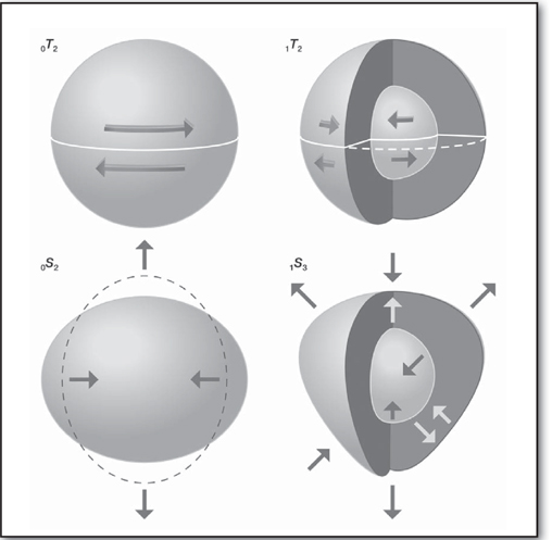
Displacements of Earth in four types of free vibrations. Encyclopædia Britannica, Inc.
Sometimes earthquakes are large enough to cause the whole Earth to ring like a bell. The deepest tone of vibration of the planet is one with a period (the length of time between the arrival of successive crests in a wave train) of 54 minutes. Knowledge of these vibrations has come from a remarkable extension in the range of periods of ground movements that can be recorded by modern digital long-period seismographs that span the entire allowable spectrum of earthquake wave periods: from ordinary P waves with periods of tenths of seconds to vibrations with periods on the order of 12 and 24 hours such as those that occur in Earth tidal movements.
The measurements of vibrations of the whole Earth provide important information on the properties of the interior of the planet. It should be emphasized that these free vibrations are set up by the energy release of the earthquake source but continue for many hours and sometimes even days. For an elastic sphere such as Earth, two types of vibrations are known to be possible. In one type, called S modes, or spheroidal vibrations, the motions of the elements of the sphere have components along the radius as well as along the tangent. In the second type, which are designated as T modes, or torsional vibrations, there is shear but no radial displacements. The nomenclature is n S l and n T l, where the letters n and l are related to the surfaces in the vibration at which there is zero motion. The subscript n gives a count of the number of internal zero-motion (nodal) surfaces, and l indicates the number of surface nodal lines.
(A) Recorded ground motion for 20 hours at Whiskeytown, California, in the large Indonesian earthquake, 1977. (B) Frequency spectrum of Earth’s oscillations from that record. Encyclopædia Britannica, Inc.
Several hundred types of S and T vibrations have been identified and the associated periods measured. The amplitudes of the ground motion in the vibrations have been determined for particular earthquakes, and, more important, the attenuation of each component vibration has been measured. The dimensionless measure of this decay constant is called the quality factor Q. The greater the value of Q, the less the wave or vibration damping. Typically, for o S 10 and o T 10, the Q values are about 250.
Recent research has shown that observations of long-period oscillations of Earth discriminate fairly finely between different Earth models. In applying the observations to improve the resolution and precision of such representations of the planet’s internal structure, a considerable number of Earth models are set up, and all the periods of their free oscillations are computed and checked against the observations. Models can then be successively eliminated until only a small range remains. In practice, the work starts with existing models; efforts are made to amend them by sequential steps until full compatibility with the observations is achieved, within the uncertainties of the observations. Even so, the resulting computed Earth structure is not a unique solution to the problem.
Space vehicles have carried equipment to the surface of the Moon and Mars with which to record seismic waves, and seismologists on Earth have received telemetered signals from seismic events in both cases.
By 1969, seismographs had been placed at six sites on the Moon during the U.S. Apollo missions. Recording of seismic data ceased in September 1977. The instruments detected between 600 and 3,000 moonquakes during each year of their operation, though most of these seismic events were very small. The ground noise on the lunar surface is low compared with that of Earth, so that the seismographs could be operated at very high magnifications. Because there was more than one station on the Moon, it was possible to use the arrival times of P and S waves at the lunar stations from the moonquakes to determine foci in the same way as is done on Earth.
Moonquakes are of three types. First, there are the events caused by the impact of lunar modules, booster rockets, and meteorites. The lunar seismograph stations were able to detect meteorites hitting the Moon’s surface more than 1,000 km (600 miles) away. The two other types of moonquakes had natural sources in the Moon’s interior: they presumably resulted from rock fracturing, as on Earth. The most common type of natural moonquake had deep foci, at depths of 600 to 1,000 km; the less common variety had shallow focal depths.
Seismological research on Mars has been less successful. Only one of the seismometers carried to the Martian surface by the U.S. Viking landers during the mid-1970s remained operational, and only one potential marsquake was detected in 546 Martian days.
A number of other important concepts related to the study of earthquakes are presented below. The majority of these terms describe the kinds of locations in which earthquakes are likely to occur or the instrumentation used to measure these phenomena.
This zone of earthquake epicentres (points on the surface directly above the foci, or origination points, of earthquakes) surrounds the Pacific Ocean and coincides with tectonic plate boundaries. For much of its length the belt follows chains of island arcs such as Tonga and New Hebrides, the Philippines, Japan, the Kuril Islands, and the Aleutians, or arc-shaped features, such as the Andes. Volcanoes are associated with the Circum-Pacific Belt throughout its length; for this reason this encircling Pacific Ocean belt is often called the Ring of Fire. Deep ocean troughs bound the belt on the oceanic side; continental land masses lie behind. The Circum-Pacific Belt is the source of approximately 80 percent of the world’s shallow-focus earthquakes and virtually all deep-focus earthquakes.
In geology, a fault is a planar or gently curved fracture in the rocks of Earth’s crust, where compressional or tensional forces cause relative displacement of the rocks on the opposite sides of the fracture. Faults range in length from a few centimetres to many hundreds of kilometres, and displacement likewise may range from less than a centimetre to several hundred kilometres along the fracture surface (the fault plane). In some instances, the movement is distributed over a fault zone composed of many individual faults that occupy a belt hundreds of metres wide. The geographic distribution of faults varies; some large areas have almost none, others are cut by innumerable faults.
Faults may be vertical, horizontal, or inclined at any angle. Although the angle of inclination of a specific fault plane tends to be relatively uniform, it may differ considerably along its length from place to place. When rocks slip past each other in faulting, the upper or overlying block along the fault plane is called the hanging wall, or headwall; the block below is called the footwall. The fault strike is the direction of the line of intersection between the fault plane and the surface of Earth. The dip of a fault plane is its angle of inclination measured from the horizontal.
Faults are classified according to their angle of dip and their relative displacement. Normal dip-slip faults are produced by vertical compression as Earth’s crust lengthens. The hanging wall slides down relative to the footwall. Normal faults are common; they bound many of the mountain ranges of the world and many of the rift valleys found along spreading margins of tectonic plates. Rift valleys are formed by the sliding of the hanging walls downward many thousands of metres, where they then become the valley floors.
A block that has dropped relatively downward between two normal faults dipping toward each other is called a graben. A block that has been relatively uplifted between two normal faults that dip away from each other is called a horst. A tilted block that lies between two normal faults dipping in the same direction is a tilted fault block.
Reverse dip-slip faults result from horizontal compressional forces caused by a shortening, or contraction, of the Earth’s crust. The hanging wall moves up and over the footwall. Thrust faults are reverse faults that dip less than 45°. Thrust faults with a very low angle of dip and a very large total displacement are called overthrusts or detachments; these are often found in intensely deformed mountain belts. Large thrust faults are characteristic of compressive tectonic plate boundaries, such as those that have created the Himalayas and the subduction zones along the west coast of South America.
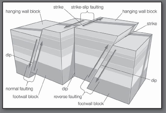
In normal and reverse faulting, rock masses slip vertically past each other. In strike-slip faulting, the rocks slip past each other horizontally. Encyclopædia Britannica, Inc.
Strike-slip (also called transcurrent, wrench, or lateral) faults are similarly caused by horizontal compression, but they release their energy by rock displacement in a horizontal direction almost parallel to the compressional force. The fault plane is essentially vertical, and the relative slip is lateral along the plane. These faults are widespread. Many are found at the boundary between obliquely converging oceanic and continental tectonic plates. A well-known terrestrial example is the San Andreas Fault, which, during the San Francisco earthquake of 1906, had a maximum movement of 6 metres (20 feet).
Oblique-slip faults have simultaneous displacement up or down the dip and along the strike. The displacement of the blocks on the opposite sides of the fault plane usually is measured in relation to sedimentary strata or other stratigraphic markers, such as veins and dikes. The movement along a fault may be rotational, with the offset blocks rotating relative to one another.
Fault slip may polish smooth the walls of the fault plane, marking them with striations called slickensides, or it may crush them to a fine-grained, claylike substance known as fault gouge; when the crushed rock is relatively coarse-grained, it is referred to as fault breccia. Occasionally, the beds adjacent to the fault plane fold or bend as they resist slippage because of friction. Areas of deep sedimentary rock cover often show no surface indications of the faulting below.
Movement of rock along a fault may occur as a continuous creep or as a series of spasmodic jumps of a few metres during a few seconds. Such jumps are separated by intervals during which stress builds up until it overcomes the frictional forces along the fault plane and causes another slip. Most, if not all, earthquakes are caused by rapid slip along faults.
The Richter scale is a widely used quantitative measure of the magnitude of an earthquake, devised in 1935 by American seismologist Charles F. Richter.
The Richter scale was originally devised to measure the magnitude of local earthquakes in southern California as recorded by a specific kind of seismograph. Current scientific practice has replaced the original Richter scale with other scales, including the body-wave magnitude scale and the moment magnitude scale, which have no restrictions regarding distance and type of seismograph used. Nevertheless, the Richter scale is still commonly cited in news reports of earthquake severity.
On the original Richter scale the smallest earthquakes measurable at that time were assigned values close to zero. Since modern seismographs can detect seismic waves even smaller than those originally chosen for zero magnitude, the Richter scale now measures earthquakes having negative magnitudes. Each increase of one unit on the scale represents a 10-fold increase in the magnitude of an earthquake–in other words, numbers on the Richter scale are proportional to the common (base 10) logarithms of maximum wave amplitudes. In theory the scale has no upper limit, but in practice no earthquake has ever been registered above magnitude 9.
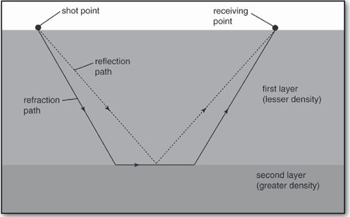
Simplified view of seismic survey methods. Encyclopædia Britannica, Inc.
A seismic belt is a narrow geographic zone on Earth’s surface along which most earthquake activity occurs. The outermost layer of Earth (lithosphere) is made up of several large tectonic plates. The edges where these plates move against one another are the location of interplate earthquakes that produce the seismic belts. Island arcs, mountain chains, volcanism, deep ocean troughs, and oceanic ridges are often features of seismic belts. The two major seismic belts are the Circum-Pacific Belt, which surrounds the Pacific Ocean, and the Alpide Belt, which stretches from the Azores through the Mediterranean and Middle East to the Himalayas and Indonesia, where it joins the Circum-Pacific Belt. A purely oceanic seismic belt lies along the mid-Atlantic ridge.
A seismic survey is a method of investigating subterranean structure, particularly as related to exploration for petroleum, natural gas, and mineral deposits. The technique is based on determinations of the time interval that elapses between the initiation of a seismic wave at a selected shop point and the arrival of reflected or refracted impulses at one or more seismic detectors. Seismic air guns are commonly used to initiate the seismic waves. This technique has largely replaced the practice of exploding dynamite underground. Electric vibrators or falling weights (thumpers) may also be employed at sites where an underground explosion might cause damage—e.g., where caverns are present. Upon arrival at the detectors, the amplitude and timing of waves are recorded to give a seismogram (record of ground vibrations).
Generally, the density of rocks near the surface of Earth increases with depth. Seismic waves initiated at the shot point may reach the receiving point by reflection, refraction, or both. When the shot point is close to the receiving point, reflected waves usually reach the receiving point first. At greater distances, however, the seismic pulse travels faster by the refraction path because its velocity is greater along the top of the lower, denser layer than it is through the upper layer; in this case, the refracted wave arrives first.
Interpretation of the depths and media reached by seismic waves thus depends on the distance between shot points and receiving points and the densities of the strata. The results of a seismic survey may be presented in the form of a cross-sectional drawing of the subsurface structures as if cut by a plane through the shot point, the detector, and the centre of Earth. Such drawings are called seismic profiles.
A seismograph is an instrument that makes a record of seismic waves caused by an earthquake, explosion, or other Earth-shaking phenomenon. Seismographs are equipped with electromagnetic sensors that translate ground motions into electrical changes, which are processed and recorded by the instruments’ analog or digital circuits. A record produced by a seismograph on a display screen or paper printout is called a seismogram. Although originally designed to locate natural earthquakes, seismographs have many other uses, such as petroleum exploration, investigation of Earth’s crust and lower layers, and monitoring of volcanic activity.
An early seismic instrument called the seismoscope made no time record of ground oscillations but simply indicated that shaking had occurred. A Chinese scholar, Chang Heng, invented such an instrument as early as 132 CE. It was cylindrical in shape with eight dragon heads arranged around its upper circumference, each with a ball in its mouth. Around the lower circumference were eight frogs, each directly under a dragon head. When an earthquake occurred, one of the balls was released from a dragon’s mouth, probably by an internal pendulum, and was caught by a frog’s mouth.
A device involving water spillage was developed in 17th-century Italy. Later a water-filled bowl and still later a cup filled with mercury were used for detecting earthquakes and tremors. In 1855 Luigi Palmieri of Italy designed a seismometer, an instrument that senses the amount of ground motion. Palmieri’s seismometer consisted of several U-shaped tubes filled with mercury and oriented toward the different points of the compass. When the ground shook, the motion of the mercury made an electrical contact that stopped a clock and simultaneously started a recording drum on which the motion of a float on the surface of mercury was registered. This device thus indicated time of occurrence and the relative intensity and duration of the ground motion.
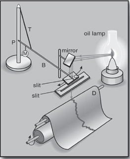
Horizontal pendulum seismograph, as invented by English seismologist John Milne in 1880. From Bulletin of the Seismological Society of America (1969), vol. 59, no. 1, p. 212
The basic problem in measuring ground motions is to attain a steady point that remains fixed when the ground moves. Various types of pendulums have been used for this purpose. The simplest type is a common pendulum in which a heavy mass is suspended by a wire or rod from a fixed point (as in a clock). Other forms are the inverted pendulum, in which a heavy mass is fixed to the upper end of a vertical rod pointed at its lower end, and the horizontal pendulum, in which a rod with a mass on its end is suspended at two points so as to swing in a nearly horizontal plane instead of a vertical plane. In 1840 a seismometer based on the common pendulum was installed near Comrie in Perthshire, Scotland.
Seismograph developments occurred rapidly in 1880 when Sir James Alfred Ewing, Thomas Gray, and John Milne, British scientists working in Japan, began to study earthquakes. Following a severe earthquake that occurred at Yokohama near Tokyo in that year, they organized the Seismological Society of Japan. Under its auspices various devices, forerunners of today’s seismograph, were invented. Among the instruments constructed in this period was Milne’s famous horizontal pendulum seismograph. In his design, a boom, to which the mass was attached, was suspended horizontally by a pivot and a silk thread fixed to a point above the pivot. A thin plate, in which a narrow slit was cut parallel to the boom, was attached to the end of the boom. A similar plate with a slit at right angles to the upper plate was fixed on the top of a box containing a recording drum. A ray of light from an oil lamp passed through both slits and formed a small spot of light on a sheet of light-sensitive graph paper (bromide paper) wrapped on the recording drum. Milne successfully used this seismograph to record several earthquakes in Japan; then, after returning to England, he established a small worldwide seismographic network using such instruments.
The horizontal pendulum seismograph was improved greatly after World War II. The Press-Ewing seismograph, developed in the United States for recording long-period waves, was widely used throughout the world. This device employed a Milne-type pendulum, but the pivot supporting the pendulum was replaced by an elastic wire to avoid friction.
If a common pendulum is free to swing in one direction and if the ground moves rapidly in the direction of freedom of the pendulum while the pendulum is motionless, the pendulum will tend to remain in place through inertia. If the ground moves back and forth (oscillates) and if the period of ground motion (the time necessary for one complete oscillation) is sufficiently shorter than the period of free oscillation of the pendulum, the pendulum will again lag, and the movement of the ground relative to the pendulum can be recorded. The magnitude of this movement is commonly amplified electrically. When the period of the pendulum is comparable to that of the ground motion, the seismograph will not exactly record Earth’s movement. The correction, however, can readily be computed mathematically.
In general, then, the seismograph is an instrument in which the relative motion of pendulum and ground is recorded. It is equally possible to take the ratio between the deflection of the pendulum and the velocity (or acceleration) of the ground. This ratio is called the velocity (or acceleration) sensitivity of the seismograph.
If free oscillation of the pendulum is not minimized, it will mask the proper recording of seismic waves. The simplest way to reduce (damp out) the free oscillation of a pendulum is to suspend it in a viscous (thick) liquid of which the resisting force is proportional to the velocity of the pendulum. In practice, the required resisting force is exerted by a special device called a damper. In an electromagnetic damper, the resisting force is created by electrical currents induced in a copper plate moving in a strong magnetic field.
The ground can move in any of three directions, two horizontal and one vertical. Because each kind of movement must be separately recorded, three pendulums, one for each direction, are needed for a complete seismograph.
Various methods of recording pendulum motion have been developed. In the mechanical method (now of historical interest only), a sheet of smoked paper was wrapped around a rotating drum, so mounted as to move with Earth. A moving pen connected to the pendulum pressed lightly on the paper. The rotating drum shifted slightly with each revolution so that recorded lines were not superimposed on each other. The drum rotated without interruption; one sheet of paper usually lasted 24 hours. Though this method was simple and economical, the seismograph had to have a heavy mass to overcome the friction between pen and paper. In consequence, some mechanical seismographs weighed one ton or more. In the more modern optical method, pendulum motion causes a mirror to move; light is reflected by this mirror onto photosensitive paper wrapped on a drum. Thus, there is no friction to affect the pendulum.
In the electromagnetic method, widely used today, a coil fixed to the mass of the pendulum moves in a magnetic field and creates an electric current. When the current is amplified electronically, high magnification is obtainable. Certain short-period seismographs of this type used for the observation of microearthquakes attain a magnification as high as 1,000,000 or more. In ordinary seismographic observation, the time of initiation of ground oscillations is recorded. Marks are placed on the seismogram once a minute; an extra one identifies the hour.
All the seismographs described so far measure oscillatory motions of the ground at a given point. The strain seismograph, in contrast, employs no pendulum, and its operation depends on changes in the distance between two points on the ground. This type of seismograph was devised in 1935.
Strong-motion seismographs, called accelerographs, are designed particularly to register intense movements of the ground, mainly for engineering purposes—i.e., antiseismic construction in earthquake-prone areas such as Japan. Strong-motion seismographs employ accelerometers as sensors, record digitally directly on magnetic tape or memory chips, and can measure ground acceleration up to twice gravity. Networks of accelerographs are now operative in several earthquake regions (e.g., California, Japan, Taiwan, Mexico), offering continuous direct recording linked to computers and the World Wide Web. Data on ground shaking are thus available within minutes of a local damaging earthquake.
A seismograph records oscillation of the ground caused by seismic waves that travel from their point of origin through Earth or along its surface. The seismogram of a nearby small earthquake is of simple pattern, showing the arrival of P waves (waves that vibrate in the direction of propagation), S waves (waves that vibrate at right angles to the direction of propagation), and surface waves. In the case of distant earthquakes or of nearby very large earthquakes, the seismogram pattern is more complicated because it shows various sorts of seismic waves that originate from one or many points but then may be reflected or refracted within Earth’s crust before reaching the seismograph. The relation between the arrival time of the P and S waves and the epicentral distance—i.e., the distance from the point of origin—is expressed by a time-distance curve, in which the arrival time is read on the vertical axis and the epicentral distance on the horizontal axis. If the arrival times of various seismic waves are read on the seismogram at a station and compared with the standard time-distance curves, the epicentral distance from that station (the distance of the centre of the earthquake from the recording station) can be determined. If the epicentral distance from at least three stations is known, the origin of the earthquake can be calculated by simple trigonometric methods.
The eruption of a volcano is commonly accompanied by many small earthquakes, especially when a volcano resumes activity after a long dormant period. Observation with sensitive seismographs therefore plays an important role in the prediction of volcanic activity. Often a strong earthquake is preceded by small earthquakes. Observation of very small tremors with sensitive seismographs is helpful in predicting disastrous earthquakes.
Seismographs sometimes detect small and long-continuing oscillations of the ground, called microseisms, that do not originate as earthquakes. The occurrence of some microseisms is related to storms at sea.
Seismographs are used for detecting remote nuclear underground tests. In this activity, the relatively faint seismic waves generated by an underground explosion must be distinguished from natural tremors. If the seismic waves generated by an explosive charge are recorded by sensitive seismographs installed at various points in the neighbourhood of the explosion, the underground structure of the site can be determined by analyzing the time-distance curves of P waves, both direct waves and those reflected or refracted at the boundaries of underground layers. Depths of underground layers, their angle of inclination, and the speed of seismic waves in each layer can be determined. Since the discovery of a large oil field in the United States by this method in 1923, seismic surveying has made rapid progress and is now used for oil and gas exploration. The improvement in the instruments and techniques achieved after World War II made it possible to determine the structure of Earth’s crust to a depth of 40 to 50 km (about 25 to 30 miles) by detonation of a small amount of explosive.
Ground motions caused by dynamite blasts in mines, quarries, and public works also can be measured by the seismograph. Preliminary examinations based on seismographic measurements make it possible to estimate the intensity of shocks and, thus, evaluate the possibilities of damage caused by a given amount of dynamite. Rock bursts, in which rocks are ejected suddenly in deep pits or tunnels, are caused by increase of stress in the surrounding rocks. Experience in mines shows that an increase of small shocks detectable by highly sensitive geophones—portable seismometers for field use—generally indicates a rock burst hazard.
Detection of vibrations on the lunar surface by seismographs is of fundamental importance in determining the internal structure, physical state, and tectonic (crustal) activity of the Moon. Moon seismographs were installed during the Apollo program starting in 1969. They contained three long-period seismometers and a single-component, short-period, vertical seismometer. Many moonquakes were recorded by these instruments. Similar instruments were placed on Mars by the Viking 1 and 2 landers in 1976 to determine the extent of seismic activity on that planet.
The modern scientific understanding of earthquakes owes much to the work of seismologists and geologists. Some of the more influential personages, such as August Edward Hough Love, who described surface waves, John Milne, who created the modern seismograph, and Charles Richter, who developed a widely used scale for assessing earthquake magnitude, are presented below.
(b. June 4, 1889, Darmstadt, Ger.—d. Jan. 25, 1960, Los Angeles, Calif., U.S.)
Beno Gutenberg was an American seismologist noted for his analyses of earthquake waves and the information they furnish about the physical properties of Earth’s interior.
Gutenberg served as a professor of geophysics and director of the seismological laboratory at the California Institute of Technology, Pasadena, from 1930 to 1957, when he retired. He worked with Charles Richter to develop a method of determining the intensity of earthquakes. Calculating the energy released by present-day shallow earthquakes, they showed that three-quarters of that energy occurs in the Circum-Pacific belt. Gutenberg wrote several books, including Earthquakes in North America (1950); he edited Internal Constitution of the Earth (1939) and, with Richter, wrote The Seismicity of the Earth (1941).
(b. April 22, 1891, Fatfield, Durham, Eng.—d. March 18, 1989, Cambridge),
Sir Harold Jeffreys was a British astronomer and geophysicist noted for his wide variety of scientific contributions.
Jeffreys was educated at Armstrong College, Newcastle-upon-Tyne (D.Sc., 1917), and St. John’s College, University of Cambridge (M.A., 1917), and was a fellow at St. John’s from 1914. He served in the Meteorological Office (1917–22), lectured in mathematics at Cambridge (1923–32), was reader in geophysics at Cambridge (1932–46), and was the university’s Plumian professor of astronomy (1945–58). He was knighted in 1953.
In his work in astronomy, Jeffreys established that the four large outer planets (Jupiter, Saturn, Uranus, and Neptune) are very cold and devised early models of their planetary structure. His other astronomical work includes research into the origin of the solar system and the theory of the variation of latitude.
In geophysics, he investigated the thermal history of Earth, was coauthor (1940) of the standard tables of travel times for earthquake waves, and was the first to demonstrate that the Earth’s core is liquid. He explained the origin of monsoons and sea breezes and showed how cyclones are vital to the general circulation of the atmosphere. Jeffreys also published seminal works on probability theory and on methods of general mathematical physics.

Sir Harold Jeffreys. Camera Press
Jeffreys was an effective critic of the mechanical feasibility of the theory of continental drift, a forerunner of modern plate tectonics. His skepticism of the possibility of convection in the Earth’s mantle carried over to strong objections to plate tectonics as well—an opposition he maintained all his life in spite of mounting geophysical evidence that the theory was correct.
Jeffreys’s honours included the Gold Medal of the Royal Astronomical Society (1937) and the Royal Medal of the Royal Society of London (1948). Among his principal works, many of which went through multiple editions in his lifetime, are The Earth: Its Origin, History and Physical Constitution (1924), Theory of Probability (1939), Earthquakes and Mountains (1935), and Methods of Mathematical Physics (1946), written with his wife, Lady Bertha Swirles Jeffreys. The Collected Papers of Sir Harold Jeffreys was published in six volumes from 1971 to 1977.
(b. April 17, 1863, Weston-super-Mare, Somerset, Eng.—d. June 5, 1940, Oxford)
Augustus Edward Hough Love, a British geophysicist and mathematician, discovered a major type of seismic wave that was subsequently named for him.
Love held the Sedleian professorship of natural philosophy at the University of Oxford from 1899 to 1940. In his analysis of earthquake waves, Love made the assumption that Earth consists of concentric layers that differ in density and postulated the occurrence of a seismic wave confined to the surface layer, or crust, of Earth. This wave would be propagated as a result of the difference in density between the crust and underlying mantle. His prediction was confirmed by recordings of the behaviour of waves in the surface layer of Earth. He proposed a method—based on measurements of Love waves—to measure the thickness of Earth’s crust. In addition to his work on geophysical theory, Love studied elasticity and wrote A Treatise on the Mathematical Theory of Elasticity, 2 vol. (1892–93).
(b. 1724, Nottinghamshire, Eng.—d. April 21, 1793, Thornhill, Yorkshire)
A British geologist and astronomer, John Michell is considered one of the fathers of seismology, the science of earthquakes.
In 1760, the year in which he was elected a fellow of the Royal Society of London, Michell finished writing Conjectures Concerning the Cause, and Observations upon the Phænomena of Earthquakes, in which he presented the conclusions from his study of the disastrous Lisbon earthquake of 1755. He showed that the focus of that earthquake was underneath the Atlantic Ocean, and he proposed erroneously that the cause of earthquakes was high-pressure steam, created when water comes into contact with subterranean fires. His contributions to astronomy included the first realistic estimate of the distance between Earth and a star and the suggestion, later verified by the English astronomer John Herschel, that binary stars are physically close to and in orbit around each other.
Michell became Woodwardian Professor of Geology at the University of Cambridge in 1762 and rector of Thornhill in 1767. In 1750 he had published a major work on artificial magnets. He may have conceived the principle of the torsion balance independently of the French physicist Charles-Augustin de Coulomb. He hoped to use this instrument to determine the mean density of Earth. Although he died before finishing his work, it was carried on by the English physicist Henry Cavendish in his determination of G, the gravitational constant (a measure of the strength of gravitation).
(b. Dec. 30, 1850, Liverpool, Eng.—d. July 30, 1913, Shide, Isle of Wight)
An English geologist and influential seismologist, John Milne developed the modern seismograph and promoted the establishment of seismological stations worldwide.
Milne worked as a mining engineer in Labrador and Newfoundland, Canada, and in 1874 served as geologist on the expedition led by Charles T. Beke, the noted British explorer and biblical scholar, to Egypt and northwestern Arabia. In 1875 Milne accepted the position of professor of geology and mining at the Imperial College of Engineering, Tokyo. He designed one of the first reliable seismographs in 1880 and traveled widely in Japan to set up 968 seismological stations for a survey of Japan’s widespread earthquakes. After many seminal earthquake studies, Milne returned to England in 1894 and established a private seismological station near Newport, Isle of Wight. His attempt in 1906 to determine the velocity of seismic waves through Earth was largely unsuccessful. He served as secretary of the Seismological Committee of the British Association and organized a worldwide network of observation stations. Many of his findings were published in his books Earthquakes (1883) and Seismology (1898).
(b. May 18, 1859, Baltimore, Md., U.S.—d. June 18, 1944, Baltimore)
Harry Fielding Reid was an American seismologist and glaciologist who in 1911 developed the elastic rebound theory of earthquake mechanics, still accepted today.
Reid was professor of applied mechanics at Johns Hopkins University, Baltimore, from 1896 until he became emeritus professor in 1930. His early career was mainly concerned with the study of the structure, composition, and movement of glaciers. Later he became involved in the study of earthquakes and earthquake-recording devices. He was first to develop a mechanism that explained how earthquakes were a result of faulting and not the reverse. He wrote an analysis of the 1906 San Francisco earthquake as part of the California State Earthquake Investigation Commission report, Mechanics of the Earthquake.
(b. April 26, 1900, near Hamilton, Ohio, U.S.—d. Sept. 30, 1985, Pasadena, Calif.)
Charles F. Richter, an American physicist and seismologist, developed the Richter scale for measuring earthquake magnitude.
Born on an Ohio farm, Richter moved with his mother to Los Angeles in 1916. He attended the University of Southern California (1916–17) and then studied physics at Stanford University (A.B., 1920) and the California Institute of Technology (Ph.D., 1928). Richter was on the staff of the Seismological Laboratory of the Carnegie Institution of Washington, Pasadena, California (1927–36), and then taught both physics and seismology at Caltech (1937–70) and worked at its Seismological Laboratory (founded in 1936).
With Beno Gutenberg (1889–1960), a German-born Caltech professor, he developed in 1935 the magnitude scale that came to be associated with his name. Based on instrumental recording of ground motion, it provided a quantitative measure of earthquake size and complemented the older Mercalli scale, which was based on an earthquake’s reported intensity. Richter also mapped out quake-prone areas in the United States, though he disparaged attempts at earthquake prediction. He wrote (with Beno Gutenberg) Seismicity of the Earth and Associated Phenomena (1949) and Elementary Seismology (1958). He also wrote the article Earthquakes for the 15th edition of Encyclopædia Britannica (first published 1974).
Earth’s surface and interior are prone to the violence caused by tectonic forces. The activities of seismic waves during earthquakes and the expulsion of molten rock, explosive gases, and ash that occur during volcanic eruptions scar and deform Earth’s surface. When people and their settlements occur within areas affected by earthquakes and volcanic eruptions, the potential for tremendous loss of life and property damage is always present. Secondary events spawned by earthquakes and volcanic eruptions, such as tsunamis and landslides, can add further misery. There are many examples of cities and regions falling victim to volcanic eruptions and massive earthquake events. Some events (such as the eruptions of Mount Toba, Mount Tambora, and Mount Pinatubo) have even affected global climate patterns.
Despite the devastation caused by these tectonic forces, the activities of earthquakes and volcanoes also recycle and remake Earth’s surface. At smaller timescales, ash and rock from volcanic eruptions become deposits of soil that can be used by plants, and lava extruded from volcanoes can add coastline. Across geologic timescales, tectonic forces are responsible for breaking continents into multiple pieces and for building mountains when continents, or parts of continents, collide. These processes can transcend geology since they can also strongly influence the evolution of life.