Getting to Know the Problem
Our friend Roberto owns a cozy little pizzeria in Berlin. Every day at noon, he checks the number of reserved seats and decides how much pizza dough to prepare for dinner. Too much dough, and it goes wasted; too little, and he runs out of pizzas. In either case, he loses money.
It’s not always easy to gauge the number of pizzas from the reservations. Many customers don’t reserve a table, or they eat something other than pizza. Roberto knows that there is some kind of link between those numbers, in that more reservations generally mean more pizzas—but other than that, he’s not sure what the exact relation is.
Roberto dreams of a program that looks at historical data, grasps the relation between reserved seats and pizzas, and uses it to forecast tonight’s pizza sales from today’s reservations. Can we code such a program for him?
Supervised Pizza
Remember what I said back in Supervised Learning? We can solve Roberto’s pizza forecasting problem by training a supervised learning algorithm with a bunch of labeled examples. To get the examples, we asked Roberto to jot down a few days’ worth of reservations and pizzas, and collected those data in a file. Here’s what the first four lines of that file look like:
| | Reservations Pizzas |
| | 13 33 |
| | 2 16 |
| | 14 32 |
| | 23 51 |
The file contains 30 lines of data. Each is an example, composed of an input variable (the reservations) and a numerical label (the pizzas). Once we have an algorithm, we can use these examples to train it. Later on, during the prediction phase, we can pass a specific number of reservations to the algorithm, and ask it to come up with a matching number of pizzas.
Let’s start with the numbers, like a data scientist would.
Making Sense of the Data
If we glance at Roberto’s examples, it seems that the reservations and pizzas are correlated. Let’s fire up a Python shell (with the python3 command) and take a deeper look.
The NumPy library has a convenient function to import whitespace-separated data from text:
| | import numpy as np |
| | X, Y = np.loadtxt("pizza.txt", skiprows=1, unpack=True) |
The first line imports the NumPy library, and the second uses NumPy’s loadtxt function to load the data from the pizza.txt file. I skipped the headers row, and I “unpacked” the two columns into separate arrays called X and Y. X contains the values of the input variable, and Y contains the labels. I used uppercase names for X and Y, because that’s a common Python convention to indicate that a variable should be treated as a constant.
Let’s peek at the data, to make sure they loaded okay. If you wish to follow along, start a Python interpreter, send the two lines given before, and then check out the first few elements of X and Y:
| => | X[0:5] |
| <= | [ 13. 2. 14. 23. 13.] |
| => | Y[0:5]) |
| <= | [ 33. 16. 32. 51. 27.] |
The numbers are consistent with Roberto’s file, but it’s still hard to make sense of them. Plot them on a chart, though, and they become clear:
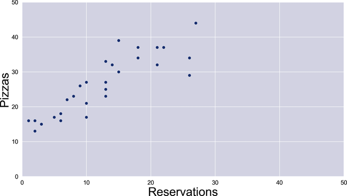
Now the correlation jumps out at us: the more reservations, the more pizzas. To be fair, a statistician might scold us for drawing conclusions from a handful of hastily collected examples. However, this is no research project—so let’s ignore the little statistician on our shoulder, and build a pizza forecaster.