Gradient Descent

Let’s look for a better train algorithm. The job of train is to find the parameters that minimize the loss, so let’s start by focusing on loss itself:

	def loss(X, Y, w, b):
	return np.average((predict(X, w, b) - Y) ** 2)

Look at this function’s arguments. X and Y contain the input variables and the labels, so they never change from one call of loss to the next. To make the upcoming discussion easier, let’s also temporarily fix b at 0. So now the only variable is w.

How does the loss change as w changes? I put together a program that plots loss for w ranging from -1 to 4, and draws a green cross on its minimum value. Check out the following graph (as usual, that code is among the book’s source code):

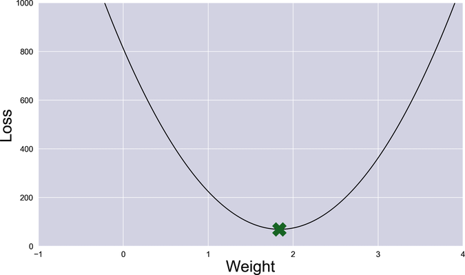
Nice curve! Let’s call it the loss curve. The entire idea of train is to find that marked spot at the bottom of the curve—the value of w that gives the minimum loss. At that w, the model approximates the data points as well as it can.

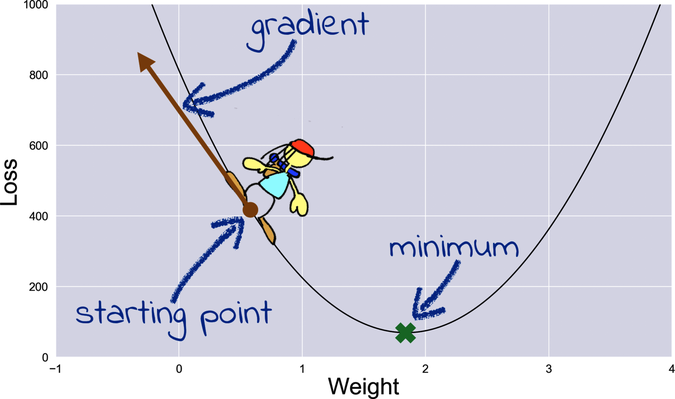
Now imagine that the loss curve is a valley, and there is a hiker standing somewhere in this valley. The hiker wants to reach her basecamp, right where the marked spot is—but it’s dark, and she can only see the terrain right around her feet. To find the basecamp, she can follow a simple approach: walk in the direction of the steepest downward slope. If the terrain doesn’t contain holes or cliffs—and our loss function doesn’t—then each steps will take the hiker closer to the basecamp.

To turn that idea into running code, we need to measure the slope of the loss curve. In mathspeak, that slope is called the gradient of the curve. By convention, the gradient at a certain point is an arrow that points directly uphill from that point, like this:

To measure the gradient, we can use a mathematical tool called “the derivative of the loss with respect to the weight,” written ∂L/∂w. More formally, the derivative at a certain point measures how the loss L changes at that point for small variations of w. Imagine increasing the weight just a tiny little bit. What happens to the loss? In the case of the diagram here, the derivative would be a negative number, meaning that the loss is decreasing. If the derivative were positive, that would mean that the loss is increasing. At the minimum point of the curve—the point marked with the cross—the curve is level, and the derivative is zero.

In the case of the diagram here, the derivative would be a negative number, meaning that the loss decreases when w increases. If the hiker were standing on the right side of the diagram, the derivative would be positive, meaning that the loss increases when w increases. At the minimum point of the curve—the point marked with the cross—the curve is level, and the derivative is zero.

Note that the hiker would have to walk in the direction opposite to the gradient to approach the minimum—so, in the case of a negative derivative like the one in the picture, she’d take a step in the positive direction. The size of the hiker’s steps should also be proportional to the derivative. If the derivative is a big number (either positive or negative), that means the curve is steep, and the basecamp is far away. So the hiker can take big steps with confidence. As she approaches the basecamp, the derivative becomes smaller, and so do her steps.

The algorithm I just described is called gradient descent, or GD for short. Implementing it requires a tiny bit of math.

A Sprinkle of Math

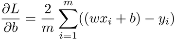
Here is how to crack gradient descent with math. First, let’s rewrite the mean squared error loss in good old-fashioned mathematical notation:

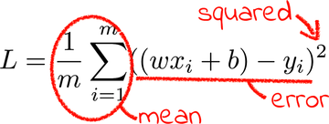
If you’re not familiar with this notation, know that the symbol stands for “sum.” Also, the m in the preceding formula stands for “the number of examples.” In English, the formula reads: add the squared errors of all the examples, from the example number one to the example number m, and divide the result by the number of examples.

Remember that the xs and ys are constants—they are the values of the input variable and the labels, respectively. m is also a constant, because the number of examples never changes. So is b, because we temporarily fixed it at zero. We’ll reintroduce b in a short while, but for the moment, the only value that varies in this formula is w.

Now we have to calculate the direction and size of the gradient—that is, the derivative of L with respect to w. If you remember calculus from school, you might be able to calculate this derivative on your own. Otherwise, don’t worry about it. Somebody already did it for us:

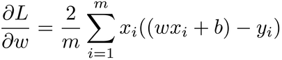
images/formulae/mse_loss_gradient_w_first.png

The derivative of the loss is somewhat similar to the loss itself, except that the power of 2 is gone, each element of the sum has been multiplied by x, and the final result is multiplied by 2. We can plug any value of w into this formula, and get back the gradient at that point.

Here’s the same formula converted to code. I fixed b at 0 as planned:

03_gradient/gradient_descent_without_bias.py

	def gradient(X, Y, w):
	return 2 * np.average(X * (predict(X, w, 0) - Y))

Now that we have a function to calculate the gradient, let’s rewrite train to do gradient descent.

Downhill Riding

Here is train, updated for gradient descent:

03_gradient/gradient_descent_without_bias.py

	def train(X, Y, iterations, lr):
	w = 0
	for i in range(iterations):
	print("Iteration %4d => Loss: %.10f" % (i, loss(X, Y, w, 0)))
	w -= gradient(X, Y, w) * lr
	return w

This version of train is much terser than the previous one. With GD, we don’t need any if. We just initialize w, and then step repeatedly in the opposite direction of the gradient. (Remember, the gradient is pointing uphill, and we want to go downhill). The lr hyperparameter is still there, but now it tells how large each step should be in proportion to the gradient.

When you do gradient descent, you have to decide when to stop it. The old version of train returned after a maximum number of iterations, or when it failed to decrease the loss further—whichever came first. With GD, the loss could in theory decrease forever, inching toward the minimum in smaller and smaller steps, without ever quite reaching it. So, when should we stop making those ever-tinier steps?

We could decide to stop when the gradient becomes small enough, because that means that we’re very close to the minimum. This code, however, follows a less refined approach: when you call train, you tell it for how many iterations to run. More iterations lead to a lower loss, but since the loss decreases progressively more slowly, at a certain point we can just decide that the additional precision isn’t worth the wait.

Later in this book (in Chapter 15, Let’s Do Development), you will learn how to choose good values for hyperparameters such as iterations and lr. For now, I just tried a bunch of different values and ended up with these ones, which seem to result in a low enough, precise enough loss:

	X, Y = np.loadtxt("pizza.txt", skiprows=1, unpack=True)
	w = train(X, Y, iterations=100, lr=0.001)
	print("\nw=%.10f" % w)

Here is what we get by running this code:

	Iteration 0 => Loss: 812.8666666667
	Iteration 1 => Loss: 304.3630879787
	Iteration 2 => Loss: 143.5265791020
	…
	Iteration 98 => Loss: 69.1209628275
	Iteration 99 => Loss: 69.1209628275

	w=1.8436928702

The loss drops at each iteration, as it should. After 100 iterations, GD got so close to the minimum that you can’t see the difference between the last two losses. It seems like our gradient descent algorithm is doing its job.

But wait—remember that we’re only using the w parameter. Let’s see what happens when we put b back in the game.

Escape from Flatland

Take a look at the loss function in math notation again:

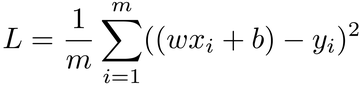
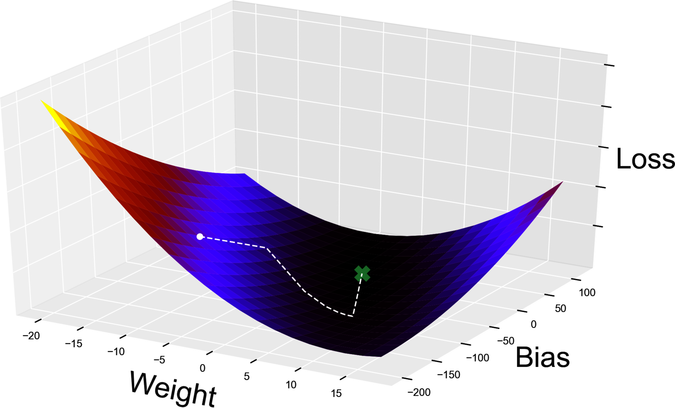
So far, we treated all the values in this function as constants, except for w. In particular, we fixed b at a value of 0. If we change b from a constant to a variable, the loss is not a two-dimensional curve anymore. Now it’s a surface as shown in the graph.

Our hiker doesn’t live in flatland anymore—she’s free to walk around in three dimensions. The two horizontal axes are the values of w and b, and the vertical axis is the value of the loss. In other words, each point on this surface represents the error of a line in our linear regression model, and we want to find the line with the lowest error: the point marked with a cross.

Even if the loss is now a surface, we can still reach its minimum point with gradient descent—only, now we need to calculate the gradient of a function of multiple variables. Fortunately for us, there is a way to do that with a technique called partial derivatives.

Partial Derivatives

Let’s see what partial derivatives are, and how they can help us. Taking a partial derivative is like slicing a function with a katana, and then calculating the derivative of the slice. (It doesn’t have to be a katana, but using a katana makes the process look cooler.) For example, when we fixed b at 0, we sliced the loss like this:

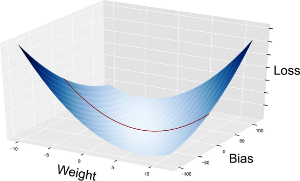
The slice shown here is the same loss curve that we plotted in Gradient Descent. It looks squashed because I used different ranges and scales for the axes, but it’s exactly the same function. For each value of b, you have one such curve, which has w as its only variable. Likewise, for each value of w you have a curve with variable b. Here is the one with w = 0 as shown in the graph.

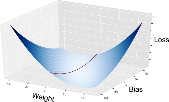
Once we have those one-dimensional slices, we can calculate the gradients on them, just like we did for the original curve. And here’s the good news: if we combine the gradient of the slices, then we get the gradient of the surface. The following graph visualizes that concept:

Thanks to partial derivatives, we just split a two-variables problem into two one-variable problems. That means that we don’t need a new algorithm to do GD on a surface. Instead, we just slice the surface using partial derivatives, and then do GD on each slice.

Math Deep Dive: Derivatives and Calculus
	The branch of mathematics that deals with gradients, derivatives, and partial derivatives is called calculus. If you want to dig deeper into calculus, check out Khan Academy.^[9] As usual, it contains way more information on the subject than you need to read this book.

In concrete, you can calculate partial derivatives by taking each variable (in our case, w and b) and pretending that it’s the only variable in the function. Just imagine that everything else is constant, and calculate the derivative with respect to that sole variable. We already did half of that work when we fixed b and calculated the derivative of L with respect to w:

Now we need to do the same, only the other way around: pretend that w is a constant, and take the derivative of L with respect to b. Feel free to calculate that partial derivative by yourself if you studied calculus. For the rest of us, here it is:

Let’s recap how GD works on a two-dimensional loss surface. Our hiker is standing at a specific spot—that is, a specific value of w and b. She’s armed with the formulas to compute the partial derivatives of L with respect to w and b. She plugs the current values of w and b into those formulas, and she gets one gradient for each variable. She applies GD to both gradients, and there you have it! She’s descending the gradient of the surface.

Enough math for this chapter. Let’s put this algorithm in code.

Putting Gradient Descent to the Test

Here is the two-variables version of our gradient descent code, with the changes marked by little arrows in the left margin:

03_gradient/gradient_descent_final.py

	import numpy as np


	def predict(X, w, b):
	return X * w + b


	def loss(X, Y, w, b):
	return np.average((predict(X, w, b) - Y) ** 2)


»	def gradient(X, Y, w, b):
»	w_gradient = 2 * np.average(X * (predict(X, w, b) - Y))
»	b_gradient = 2 * np.average(predict(X, w, b) - Y)
»	return (w_gradient, b_gradient)


	def train(X, Y, iterations, lr):
»	w = b = 0
	for i in range(iterations):
»	print("Iteration %4d => Loss: %.10f" % (i, loss(X, Y, w, b)))
»	w_gradient, b_gradient = gradient(X, Y, w, b)
»	w -= w_gradient * lr
»	b -= b_gradient * lr
»	return w, b


	X, Y = np.loadtxt("pizza.txt", skiprows=1, unpack=True)
»	w, b = train(X, Y, iterations=20000, lr=0.001)
	print("\nw=%.10f, b=%.10f" % (w, b))
	print("Prediction: x=%d => y=%.2f" % (20, predict(20, w, b)))

The gradient function now returns the partial derivatives of the loss with respect to both w and b. Those values are used by train to update both w and b, at the same time. I also bumped up the number of iterations, because the program takes longer to get close to the minimum now that it has two variables to tweak.

Let’s make an apples-to-apples comparison between this new version of the program and the one from the previous chapter. First, let’s run the earlier version with plenty of iterations and a pretty low lr of 0.0001, to get four decimal digits of precision:

	…
	Iteration 157777 -> Loss: 22.842737

	w=1.081, b=13.171
	Prediction: x=20 => y=34.80

Our new GD-based implementation runs circles around that result. With just 20,000 iterations, we get:

	…
	Iteration 19999 => Loss: 22.8427367616

	w=1.0811301700, b=13.1722676564
	Prediction: x=20 => y=34.79

Higher precision in almost one tenth of the iterations. Good stuff! This faster, more precise learner might be wasted for our pizza forecasting problem—after all, nobody buys one hundredth of a pizza. However, that additional speed will prove essential to tackle more advanced problems.

Finally, I wrote a quick visualization program to plot the algorithm’s path, from an arbitrary starting point to the minimum loss. I tried to give you an intuitive understanding of gradient descent in the previous few pages, but nothing beats watching it in motion as shown in the graph.

The hiker didn’t take the optimal route to the basecamp, because she couldn’t know that route in advance. Instead, she let the slope of the loss function guide her every step. After two abrupt changes of direction, she finally reached the bottom of the valley, and proceeded along a gently sloping trail down to the basecamp.

When Gradient Descent Fails

GD doesn’t give you many guarantees. By using it, we could follow a longer route than the shortest possible one. We could step past the basecamp, and then have to backtrack. We could even step further away from the basecamp, as the crow flies.

There are also a few unlucky cases where gradient descent might miss its target entirely. One such case has to do with the learning rate, and we’ll explore it in the Hands On exercise at the end of this chapter. Most GD failures, however, have to do with the shape of the loss surface.

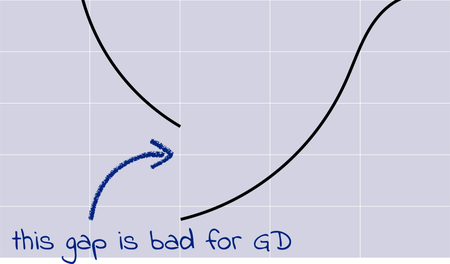
With some imagination, you can probably think of a surface that trips up the hiker on her way to the basecamp. What if the loss surface includes a sudden cliff like the one in following graph, and the hiker ends up making her best Wile E. Coyote impression?

Here is another example: what if the hiker reaches a local minimum, like the one in this graph, instead of the global minimum that it’s supposed to reach?

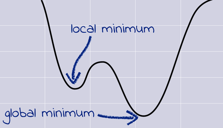
The gradient at the bottom of the local minimum is zero. If gradient descent gets in there, it gets stuck.

Long story short, GD works well as long as the loss surface has a few characteristics. In mathspeak, a good loss function should be convex (meaning that it doesn’t have bumps that result in local minima); continuous (meaning that it doesn’t have vertical cliffs or gaps); and differentiable (meaning that it’s smooth, without cusps and other weird spots where you cannot even calculate a derivative). Our current loss function ticks all those boxes, so it’s ideal for GD. Later on, we will apply GD to other functions, and we will vet those functions for such prerequisites.

GD is also the main reason why we implemented our loss with the mean squared error formula. We could have used the mean absolute value of the error—but the mean absolute value doesn’t work well with GD, because it has a non-differentiable cusp around the value 0. As a bonus, squaring the error makes large errors even larger, creating a really steep surface as you get further away from the minimum. In turn, that steepness means that GD blazes toward the minimum at high speed. Because of both its smoothness and its steepness, the mean squared error is a great fit for GD.