Upgrading the Learner

After this mathematical detour, we can come back to the work at hand. We want to upgrade our learning program to deal with multiple input variables. Let’s make a plan of action so that we don’t get lost in the process:

First, we’ll load and prepare the multidimensional data, so that we can feed them to the learning algorithm.
After preparing the data, we’ll upgrade all the functions in our code to use the new model: we’ll switch from a line to a more generic weighted sum, as I described in Adding More Dimensions.

Let’s step through this plan. Feel free to type the commands in a Python interpreter and make your own experiments. If you don’t have an interpreter handy, fear not: I will show you the output of all important commands (sometimes slightly edited, to spare space).

Preparing Data

I wish I could tell you that ML is all about building amazing AIs and looking cool. The reality is that a large part of the job is preparing data for the learning algorithm. To do that, let’s start from the file that contains our dataset:

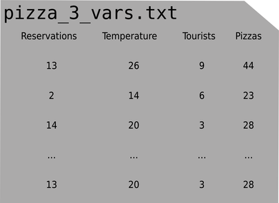
In the previous chapters, this file had two columns, which we loaded into two arrays with NumPy’s loadtxt—and that was it. Now that we have multiple input variables, X needs to become a matrix, like this:

Each row in X is an example, and each column is an input variable.

If we load the file with loadtxt, like we did before, we’ll get a NumPy array for each column:

	import numpy as np
	x1, x2, x3, y = np.loadtxt("pizza_3_vars.txt", skiprows=1, unpack=True)

Arrays are NumPy’s killer feature. They’re very flexible objects that can represent anything from a scalar (a single number) to a multidimensional structure. That same flexibility, however, makes arrays somewhat hard to grasp at first. I’ll show you how to mold those four arrays into the X and Y variables that we want—but when you get around to do this on your own, you’ll probably want to keep NumPy’s documentation handy.

To see which dimensions an array has, we can use its shape operation:

x1.shape # => (30, )

All four columns have 30 elements, one for each example in pizza_3_vars.txt. That dangling comma is NumPy’s way of saying that these arrays have just one dimension. In other words, they’re what you probably think about when you hear the word “array,” as opposed to “matrix.”

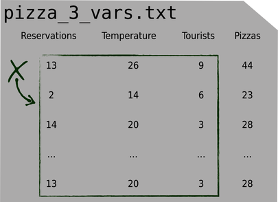
Let’s build the X matrix by joining the first three arrays together:

	X = np.column_stack((x1, x2, x3))
	X.shape # => (30, 3)

Here are the first two rows of X:

X[:2] # => array([[13., 26., 9.], [2., 14., 6.]])

NumPy’s indexes are powerful, and sometimes confusing. The notation [:2] in this code is a shortcut for [0:2], that means “the rows with index from zero to 2, excluded”—that is, the first two rows.

Now that we took care of X, let’s look at y, that still has that one-dimensional (30, ) shape. Here is one trick that saved my bottom multiple times: avoid mixing NumPy matrices and one-dimensional arrays. Code that involves both can have surprising behavior. For this reason, as soon as you have a one-dimensional array, it’s a good idea to reshape it into a matrix with the reshape function:

Y = y.reshape(-1, 1)

reshape takes the dimensions of the new array. If one dimension is -1, then NumPy will set it to whatever makes the other dimensions fit. So the preceding line means: “reshape Y so that it’s a matrix with 1 column, and as many rows as you need to fit the current elements.” The result is a (30, 1) matrix:

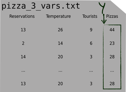
Y.shape # => (30, 1)

So now we have our data neatly arranged into an X matrix for input variables, and a Y matrix for labels. Preparing data… check! Let’s move to update the functions of our learning system, starting with the predict function.

Upgrading Prediction

Now that we have multiple input variables, we need to change the prediction formula—from the simple equation of a line, to a weighted sum:

ŷ = x1 * w1 + x2 * w2 + x3 * w3 + …

You might have noticed that something is missing in this formula. To simplify it, I temporarily removed the bias b. It will be back soon.

Now we can translate the weighted sum to a multidimensional version of predict. As a reminder, here is the old mono-dimensional predict (without the bias):

	def predict(X, w):
	return X * w

The new predict should still take X and w—but those variables have more dimensions now. X used to be a vector of m elements, where m is the number of examples. Now X is a matrix of (m, n), where n is the number of input variables. In the specific case that we’re tracking now, we have 30 examples and 3 input variables, so X is a (30, 3) matrix.

What about w? Just as we need one x per input variable, we also need one w per input variable. Different from the xs, though, the ws will be the same for each example. So we could make the weights a matrix of (n, 1), or a matrix of (1, n). For reasons that will become clear in a moment, it’s better to make it (n, 1): one row per input variable, and a single column.

Let’s initialize this matrix of (n, 1). Do you remember that we used to initialize w at zero? Now w is a matrix, so we must initialize all its elements to zeros. NumPy has a zeros function for that:

	w = np.zeros((X.shape[1], 1))
	w.shape # => (3, 1)

Remember that X.shape[0] is the number of rows in X, and X.shape[1] is the number of columns. The code here says that w has as many rows as the columns in X—in our case, 3.

And this is where matrix multiplication finally becomes useful. Look back at the weighted sum:

ŷ = x1 * w1 + x2 * w2 + x3 * w3

If X had just one row, this formula would be the multiplication of X by w:

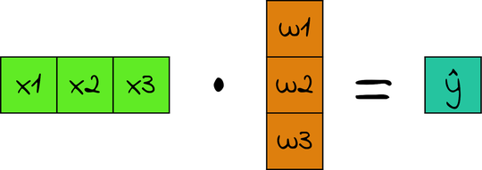
In our case, X doesn’t have one row. It has one row for each example—a (30, 3) matrix. When we multiply X by w, which is (3, 1), we get a (30, 1) matrix: one row per example, and a single column that contains the prediction for that example. In other words, a single matrix multiplication gets us the predictions for all the examples in one fell swoop!

So it turned out that rewriting prediction for multiple input variables is as simple as multiplying X and w, with a little help from NumPy’s matmul function:

	def predict(X, w):
»	return np.matmul(X, w)

It took us a while to get through this tiny function. Also, we cut a corner by temporarily ignoring the bias, which I’ll reintroduce later. So far, however, the result was worth it: predict implements the model of multiple linear regression in a single teeny line of code.

Upgrading the Loss

Moving on to the loss function—remember that we used the mean squared error to calculate the loss, like this:

	def loss(X, Y, w):
	return np.average((predict(X, w) - Y) ** 2)

Once again, I removed the bias b from loss, so that we have one less thing to worry about. We’ll reintroduce the bias in a short while. First, let’s see how we should change this stripped-down version of loss to accomodate multiple dimensions.

I remember how frustrated I got with matrix operations when I wrote my first ML programs. Matrix dimensions, in particular, never seemed to add up. With time, I learned that matrix dimensions could actually be my friends: if I tracked them carefully, they could help me piece my code together. Let’s do the same here: we can use matrix dimensions to guide us through the code.

Let’s start from the labels. We have two matrices of labels in the previous code: Y, that contains the ground truth from the dataset, and the y_hat matrix calculated by predict. Both Y and y_hat are (m, 1) matrices, meaning that they have one row for example, and one column. In our case, we have 30 examples, so they’re (30, 1). If we subtract Y from y_hat, NumPy checks that the two matrices have the same size, and subtracts each element of Y from each element of y_hat. The result is still (30, 1).

Then we want to square all the elements in this (30, 1) matrix. Because the matrix is implemented as a NumPy array, we can make use of a feature of NumPy called broadcasting, which we already used in the previous chapters: when we apply an arithmetic operation to a NumPy array, the operation is “broadcast” over each element of the array. In other words, we can square the entire matrix, and NumPy dutifully applies the “square” operation to each of its elements. The result of this operation is a matrix of squared errors, and is still (30, 1).

Finally, we call average, which averages all the elements in the matrix, returning a single scalar number:

	a_number = loss(X, Y, w)
	a_number.shape # => ()

The empty parentheses are NumPy’s way of saying: “this is a scalar, so it has no dimensions.”

Here’s the bottom line: we don’t need to change the way we calculate the loss at all. Our mean squared error code works with multiple input variables just as well as it did with one variable.

Upgrading the Gradient

We just have one last thing to do: we need to upgrade the gradient of the loss to multiple variables. I’ll cut straight to the chase and give you a matrix-based version of the gradient function:

	def gradient(X, Y, w):
	return 2 * np.matmul(X.T, (predict(X, w) - Y)) / X.shape[0]

X.T means “X transposed”—the operation that we talked about in Transposing Matrices.

See “Of Gradients and Matrices” on ProgML.

It took me a while to go from the old version of gradient to this new matrix-based one. For once, I won’t give you all the details about this function, simply because they’d take up too much space—but if you’re curious, you can read them on the book’s companion site, ProgML.^[11] If you’re so inclined, you can even check by yourself that this new version of gradient is just the same as the older gradient, except that it works with multiple input variables.

Putting It All Together

Let’s check that we have everything in order:

We wrote the code that prepares the data.
We upgraded predict.
We came to the conclusion that there is no need to upgrade loss.
We upgraded gradient.

Check… check… check… and check. We can finally apply all those changes to our learning program:

04_hyperspace/multiple_regression_without_bias.py

	import numpy as np


	def predict(X, w):
»	return np.matmul(X, w)


	def loss(X, Y, w):
	return np.average((predict(X, w) - Y) ** 2)


	def gradient(X, Y, w):
»	return 2 * np.matmul(X.T, (predict(X, w) - Y)) / X.shape[0]


	def train(X, Y, iterations, lr):
»	w = np.zeros((X.shape[1], 1))
	for i in range(iterations):
	print("Iteration %4d => Loss: %.20f" % (i, loss(X, Y, w)))
	w -= gradient(X, Y, w) * lr
	return w


»	x1, x2, x3, y = np.loadtxt("pizza_3_vars.txt", skiprows=1, unpack=True)
»	X = np.column_stack((x1, x2, x3))
»	Y = y.reshape(-1, 1)
»	w = train(X, Y, iterations=100000, lr=0.001)

We took quite a few pages to get it done, but this code is very similar to the code from the previous chapter. Aside from the part that loads and prepares the data, we changed just three lines. Also note that the functions are generic: not only they can process Roberto’s three-variables dataset—they’d work just as well with an arbitrary number of input variables.

If we run the program, here’s what we get:

	Iteration 0 => Loss: 1333.56666666666660603369
	Iteration 1 => Loss: 151.14311361881479456315
	Iteration 2 => Loss: 64.99460808656147037254
	…
	Iteration 99999 => Loss: 6.89576133146784187034

The loss decreases at each iteration, and that’s a hint that the program is indeed learning. However, our job isn’t quite done yet: you might remember that we removed the bias parameter in the beginning of this discussion, to make things easier—and we know that we shouldn’t expect good predictions without the bias. Fortunately, putting the bias back in is easier than you might think.