Invasion of the Sigmoids
Even though linear regression isn’t a natural fit for binary classification, that doesn’t mean that we have to scrap our linear regression code and start from scratch. Instead, we can adapt our existing algorithm to this new problem, using a technique that statisticians call logistic regression.
Let’s start by looking back at ŷ, the weighted sum of the inputs that we introduced in Adding More Dimensions:
| | ŷ = x1 * w1 + x2 * w2 + x3 * w3 + … |
In linear regression, ŷ could take any value. Binary classification, however, imposes a tight constraint: ŷ must not drop below 0, nor raise above 1. Here’s an idea: maybe we can find a function that wraps around the weighted sum, and constrains it to the range from 0 to 1—like this:
| | ŷ = wrapper_function(x1 * w1 + x2 * w2 + x3 * w3 + …) |
Let me repeat what the wrapper_function does. It takes whatever comes out of the weighted sum—that is, any number—and squashes it into the range from 0 to 1.
We have one more requirement: the function that we’re looking for should work well with gradient descent. Think about it: we use this function to calculate ŷ, then we use ŷ to calculate the loss, and finally we descend the loss with gradient descent. For the sake of gradient descent, the wrapper function should be smooth, without flat areas (where the gradient drops to zero) or gaps (where the gradient isn’t even defined).
To wrap it up, we want a function that smoothly changes across the range from 0 to 1, without ever jumping or flatlining. Something like this:
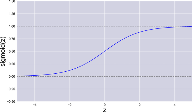
As it happens, this is a well-known function that we can use. It’s called the logistic function, and it belongs to a family of S-shaped functions called sigmoids. Actually, since “logistic function” is a mouthful, people usually just call it the “sigmoid,” for short. Here is the sigmoid’s formula:
The greek letter sigma (σ) stands for “sigmoid.” I also used the letter z for the sigmoid’s input, to avoid confusion with the system’s inputs x.
The formula of the sigmoid is hard to grok intuitively, but its picture tells us everything that we need to know. When its input is 0, the sigmoid returns 0.5. Then it quickly and smoothly falls toward 0 for negative numbers, and raises toward 1 for positive numbers—but it never quite reaches those two extremes. In other words, the sigmoid squeezes any value to a narrow band ranging from 0 to 1, it doesn’t have any steep cliffs, and it never goes completely flat. That’s the function we need!
Let’s return to the code and apply this newfound knowledge.
Confidence and Doubt
I took the formula of the sigmoid and converted it to Python, using NumPy’s exp function to implement the exponential. The result is one-line function:
| | def sigmoid(z): |
| | return 1 / (1 + np.exp(-z)) |
As usual with NumPy-based functions, sigmoid takes advantage of broadcasting: the z argument can be a number, or a multidimensional array. In the second case, the function will return an array that contains the sigmoids of all the elements of z.
Then I went back to the prediction code—the point where we used to calculate the weighted sum. The original function looked like this:
| | def predict(X, w): |
| | return np.matmul(X, w) |
I modified that function to pass the result through the sigmoid function:
| | def forward(X, w): |
| | weighted_sum = np.matmul(X, w) |
| | return sigmoid(weighted_sum) |
Later in this book, we’ll see that this process of moving data through the system is also called forward propagation, so I renamed the predict function to forward.
The result of forward is our prediction ŷ, that is a matrix with the same dimensions as the weighted sum: one row per example, and one column. Only, each element in the matrix is now constrained between 0 and 1.
Intuitively, you can see the values of y_hat as forecasts that can be more or less certain. If a value is close to the extremes, like 0.01 or 0.98, that’s a highly confident forecast. If it’s close to the middle, like 0.51, that’s a very uncertain forecast.
During the training phase, that gradual variation in confidence is just what we need. We want the loss to change smoothly, so that we can slide over it with gradient descent. Once we switch from the training phase to the classification phase, however, we don’t want the system to beat around the bush anymore. The labels that we use to train the classifier are either 0 or 1, so the classification should also be a straight 0 or 1. To get that unambiguous answer, during the classification phase we can round the result to the nearest integer, like this:
| | def classify(X, w): |
| | return np.round(forward(X, w)) |
This function could be named predict, like we used earlier, or classify. In the case of a classifier, the two words are pretty much synonyms. I opted for classify to highlight the fact that we’re not doing linear regression anymore, because now we’re forecasting a binary value.
It seems that we’re making great progress toward a classification program… except for a minor difficulty that we’re about to face.
Smoothing It Out
By adding the sigmoid to our program, we introduced a subtle problem: we made gradient descent less reliable. The problem happens when we update the loss function in our system to use the new classification code:
| | def mse_loss(X, Y, w): |
| | return np.average((forward(X, w) - Y) ** 2) |
At first glance, this function is almost identical to the loss function that we had before: the mean squared error of the predictions compared with the actual labels. The only difference from the previous loss is that the function that calculates the predicted labels ŷ has changed, from predict to forward.
That change, however, has far-reaching consequence. forward involves the calculation of a sigmoid, and because of that sigmoid, this loss isn’t the same loss that we had before. Here is what the new loss function looks like:
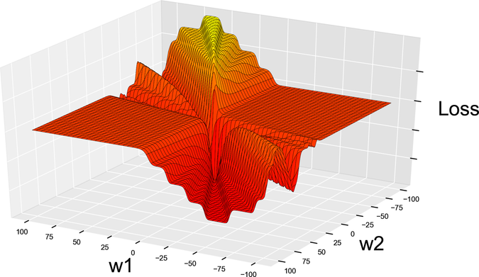
Looks like we have a problem here. See those deep canyons leading straight into holes? We mentioned those holes when we introduced gradient descent—they’re the dreaded local minima. Remember that the goal of gradient descent is to move downhill? Now consider what happens if GD enters a local minimum: since there is no “downhill” at the bottom of a hole, the algorithm stops there, falsely convinced that it’s reached the global minimum that it was aiming for.
Here is the conclusion we can take from looking at this diagram: if we use the mean squared error and the sigmoid together, the resulting loss has an uneven surface littered with local minima. Such a surface is hard to navigate with gradient descent. We’d better look for a different loss function with a smoother, more GD-friendly surface.
We can find one such function in statistics textbooks. It’s called the log loss, because it’s based on logarithms:
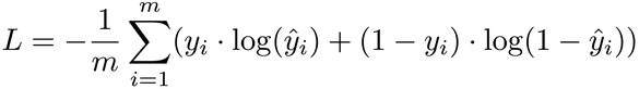
The log loss formula might look daunting, but don’t let it intimidate you. Just know that it behaves like a good loss function: the closer the prediction ŷ is to the ground truth y, the lower the loss. Also, the formula looks more friendly when turned into code:
| | def loss(X, Y, w): |
| | y_hat = forward(X, w) |
| | first_term = Y * np.log(y_hat) |
| | second_term = (1 - Y) * np.log(1 - y_hat) |
| | return -np.average(first_term + second_term) |
If you’re willing to give it a try, you’ll find that the log loss is simpler than it looks. Remember that each label in the matrix Y is either 0 or 1. For labels that are 0, the first_term is multiplied by 0, so it disappears. For labels that are 1, the second_term disappears, because it’s multiplied by (1 - Y). So each element of Y contributes only one of the two terms.
Let’s plot the log loss and see what it looks like:
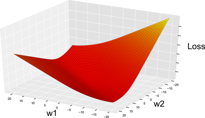
Nice and smooth! No canyons, flat areas, or holes. From now on, this will be our loss function.
Updating the Gradient
Now that we have a brand-new loss function, let’s look up its gradient. Here is the partial derivative of the log loss with respect to the weight, straight from the math textbooks:
If you have good memory, this gradient might look familiar. In fact, it closely resembles the gradient of the mean squared error that we used so far:
See how similar they are? This means that we can take our previous gradient function…
| | def gradient(X, Y, w): |
| | return 2 * np.matmul(X.T, (predict(X, w) - Y)) / X.shape[0] |
…and quickly convert it to the new formula:
| | def gradient(X, Y, w): |
| | return np.matmul(X.T, (forward(X, w) - Y)) / X.shape[0] |
With this, we’re done converting our system from linear regression to classification. Let’s take a moment to see how that change impacted the system’s model.
What Happened to the Model Function?
Back when we did linear regression, our model was a straight line, a plane, or a higher-dimensional hyperplane. In the last few sections, we changed that model by wrapping it in a sigmoid. Let’s see what the new model looks like.
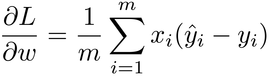
To visualize the new model, I wrote a script that trains the classifier on the first column of data in Roberto’s file, and then plots the forward function. Here is the result:
Passing the weighted sum through the sigmoid turned a straight line into something more sigmoid-y. At a glance, you can tell that this curved shape fits the data better than a line ever could. A statistician could also prove mathematically that this model is more stable in the presence of outliers.
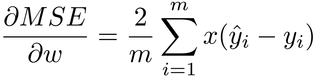
We just plotted the output of forward—the model used by the classifier during training. When it comes time to predict a label, however, the classifier passes that model through the classify function, resulting in a sharper shape as shown in the next graph:
Below a certain threshold, which in this example seems to be around 12, the value of the model is under 0.5, and classify rounds it to 0. Above that threshold, the value of the model is over 0.5, and classify rounds it to 1. The result is a stepwise model function. The job of the training phase is to stretch and shift this curve, and ultimately set the threshold where the output switches from 0 to 1.
When you add another input variable, the model function looks similar—but now it’s three-dimensional, like the graph.
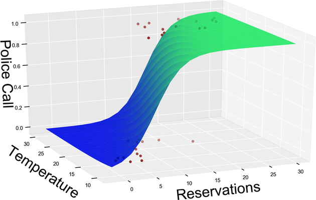
Once again, where we used to have a linear surface such as a plane, we now have a curved surface. The value of this surface gets clipped to either 0 or 1 to predict a binary label. If we add more input variables to the data, the same process happens—but the model becomes higher-dimensional, and we cannot visualize it anymore.
To be clear, the diagrams I just showed you have nothing to do with the loss curves that you’ve seen in Smoothing It Out. These plots visualize the model, while the earlier plots visualized the loss of the model. Even if these two functions are different, however, they’re related. In particular, if the model function contained sudden jumps, so would the loss. In the interest of gradient descent, it’s a good thing that the model function looks silky smooth.
Now that you’ve seen what the classifier’s model looks like, it’s time to put it through its paces. Let’s run that code.