Enter the Perceptron

To understand what a perceptron is, let’s take a look back at the binary classifier we wrote in Chapter 6, ​Getting Real​. That program sorted MNIST characters into two classes: “5” and “not a 5.” The following picture shows one way to look at it:

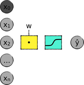
This diagram tracks an MNIST image through the system. The process begins with the input variables, from x₁ to x_n. In the case of MNIST, the input variables are the 784 pixels of an image. To those, we added a bias x₀, with a constant value of 1. I colored it a darker shade of gray, to make it stand apart from other input variables.

The next step—that yellow square—is the weighted sum of the input variables. It’s implemented as a multiplication of matrices, so I marked it with the “dot” sign.

The weighted sum flows through one last function—the light blue square. In general, this is called the activation function, and can be different for different learning systems. In our system, we used a sigmoid. The output of the sigmoid is the predicted label ŷ, ranging from 0 to 1.

During training, the system compares the prediction ŷ with the ground truth to calculate the next step of gradient descent. During classification, it snaps the value of ŷ to one of its extremes—either 1 or 0, meaning “5” and “not a 5,” respectively.

The architecture I just described is the perceptron, the original supervised learning system.

The Textbook Perceptron

If you look it up on Wikipedia, you’ll see that the textbook perceptron is actually simpler than the variant I discuss in this chapter. Instead of gradient descent, the perceptron uses a simpler algorithm, similar to the one we implemented in Chapter 2, ​Your First Learning Program​.

Since it doesn’t use gradient descent, the vanilla perceptron doesn’t need an activation function with a smooth gradient such as the sigmoid. Instead, it can get away with a simple “step” function that snaps the value of the weighted sum to either 1 or 0, depending on whether it’s positive or negative.