Bending the Boundary

Let’s switch from the perceptron to the neural network. What does its decision boundary look like?

If you bother to try the neural network on the linearly separable dataset, you’ll find that it gets the same perfect accuracy as the perceptron, and a similarly straight decision boundary. On the second dataset, however, things get interesting.

Here’s the code that trains the neural network on the non-linearly separable dataset:

12_classifiers/plot_neural_network_boundary.py

​	​import​ ​numpy​ ​as​ ​np​
​	​import​ ​neural_network​ ​as​ ​nn​
​	x1, x2, y = np.loadtxt(​'non_linearly_separable.txt'​, skiprows=1, unpack=True)
​	X_train = X_test = np.column_stack((x1, x2))
​	Y_train_unencoded = Y_test = y.astype(int).reshape(-1, 1)
​	Y_train = one_hot_encode(Y_train_unencoded)
​	w1, w2 = nn.train(X_train, Y_train,
​	X_test, Y_test,
​	n_hidden_nodes=10, iterations=100000, lr=0.3)

That’s pretty much the same code that we used to train the perceptron, with a few minor differences. Note that it doesn’t add a bias column to the data, as the network’s code takes care of that. As ever, I tried a few different values for the hyperparameters n_hidden_nodes, iterations, and lr. I ended up with the values here, which seem like a good compromise between training time and accuracy.

Here are the results:

​	Iteration: 0, Loss: 0.65876824, Accuracy: 64.00%
​	Iteration: 1, Loss: 0.65505330, Accuracy: 64.00%
​	…
​	Iteration: 99999, Loss: 0.05917079, Accuracy: 97.00%

Now we’re talking! The reason for that increased accuracy becomes evident if you visualize the neural network’s model.

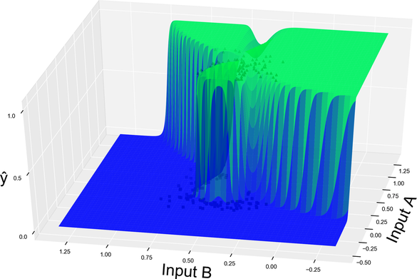
And here is a similar diagram in two dimensions, showing the neural network’s decision boundary:

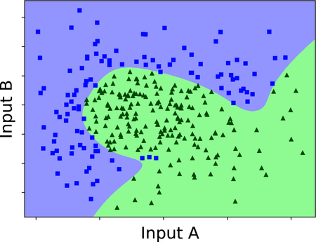
We came to the second important point of this chapter: a neural network can bend its model and decision boundary in ways that a perceptron can’t. In the case that we’re looking at, the network did a decent job of bending the boundary to separate blue squares and green triangles, leaving just a handful of misclassified points.

Check out “The Math of Multiple Layers” on ProgML.

Intuitively, a neural network’s boundary-twisting powers come from its multiple layers. The perceptron boils down to a simple weighted sum followed by a sigmoid—and that means that its model always ends up looking like a sigmoid. By chaining additional perceptrons, the neural network gets rid of that limitation. If you want a more formal explanation of why multiple layers allow the network to create bumpy models, you’ll find one on the ProgML^[20] site.

Now you know, having seen it with your own eyes, why neural networks leave perceptrons in the dust.