The Echidna Dataset

Do you remember the concept of a decision boundary, introduced back in Tracing a Boundary? Soon enough, you’ll see how a neural network’s decision boundary changes as you add a fourth layer. For that purpose, I prepared a dataset that’s twisty, but also easy to visualize. Here it is:

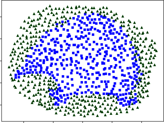
This dataset has two input variables and two classes, visualized here as squares and triangles. If you happen to be a fan of marsupials, you might notice that the dataset happens to be shaped like an echidna:^[22]

My wife and I still remember an unexpected encounter with a wild echidna on a trip to Australia. Let’s not mince words: echidnas are cool.

I saved the Echidna dataset to a file named echidna.txt. I also wrote an echidna.py file that does the same job as the mnist.py file from earlier chapters. It loads the data and the labels into two variables named X and Y, and also splits it into training, validation, and test sets:

=>	import echidna as data
=>	data.X.shape
<=	(855, 2)
=>	data.X[0:3]
<=	array([[ 0.01653543, 0.42533333],
	[ 0.14566929, -0.332 ],
	[ 0.19133858, -0.47866667]])
=>	data.Y[0:3]
<=	array([[0],
	[1],
	[1]])
=>	data.X_train.shape
<=	(285, 2)
=>	data.Y_train.shape
<=	(285, 1)

We won’t use the test set in this chapter, but the training and validation sets will become useful soon.

Now let’s build a neural network that learns the Echidna dataset.