Making It Deep

Let’s add one more layer to our three-layered neural network:

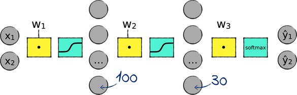
Each of the four layers in this deeper network comes with its own set of weights and its own activation function. The number of nodes in the new layer is yet one more hyperparameter, and we should be ready to tune it if we want the best results. To begin with, I set this value at 30.

Let’s turn this plan into code. That’s where using Keras really pays off, as adding this layer is a matter of adding one line of code to the model:

16_deeper/network_deep.py

	model = Sequential()
	model.add(Dense(100, activation='sigmoid'))
»	model.add(Dense(30, activation='sigmoid'))
	model.add(Dense(2, activation='softmax'))

That’s all we need. Let’s run this deeper network and see whether it fares better than the three-layered network we used before:

	Using TensorFlow backend.
	Train on 285 samples, validate on 285 samples
	Epoch 1 - loss: 0.7111 - acc: 0.4947 - val_loss: 0.6967 - val_acc: 0.4807
	…
	Epoch 30000 - loss: 0.0056 - acc: 1.0000 - val_loss: 0.7029 - val_acc: 0.8982

And here is the neural network’s decision boundary:

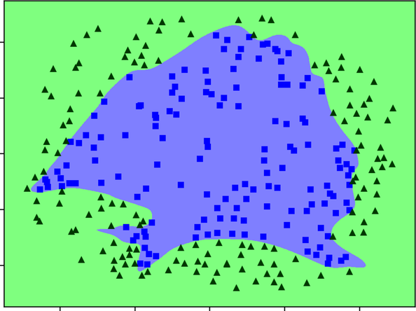
Take a moment to look at the numbers and the previous diagram. What do you think of them? Do you notice anything specifically?

At a glance, you might think that this network is amazingly successful. Its decision boundary is exceptionally good at tracking the fine details of the Echidna training set, contouring even the tiniest details to separate squares and triangles with uncanny precision. As a result, the network sports a perfect accuracy of 1 on the training set—which means that it nails the label on 100% of the training examples.

Do a double take, however, and you’ll notice something distressing: while this network is perfectly accurate on the training set, it doesn’t even come close to that perfection on the validation set. In fact, with 89.92% accuracy, this deep network does worse than its shallow counterpart on the validation set!

Let’s take a deep breath and consider what we learned from this little experiment.