Regularizing the Model

You learned three important concepts in the previous section:

• Powerful neural networks tend to overfit.
• Simple neural networks tend to underfit.
• You should strike a balance between the two.

Here is a general strategy to strike that balance: start with an overfitting model function that tracks tiny fluctuations in the data, and progressively make it smoother until you hit a good middle ground. That idea of smoothing out the model function is called “regularization,” and is the subject of this section.

In the previous chapter, we took the first step of the process I just described: we created a deep neural network that overfits the data at hand. Let’s take a closer look at that network’s model, and afterwards we’ll see how to make it smoother.

Reviewing the Deep Network

To gain more insight into overfitting, I made a few changes to our deep neural network from the previous chapter. Here’s the updated training code. The rest of the code didn’t change, so I skipped it:

17_overfitting/network_deep.py

​	​import​ ​losses​
​
​	history = model.fit(X_train, Y_train,
​	validation_data=(X_validation, Y_validation),
​	epochs=30000, batch_size=25)
​
​	boundary.show(model, data.X_train, data.Y_train,
​	title=​"Training set"​)
​	boundary.show(model, data.X_validation, data.Y_validation,
​	title=​"Validation set"​)
​	losses.plot(history)

The original network visualized the decision boundary superimposed over the validation set. I added a second diagram that shows the same boundary over the training set. Besides, I also plotted the history of the losses during training. Conveniently, Keras’s model.fit() already returns an object that contains that history—so I just had to write a utility to visualize it, that I called losses.py.

After adding this instrumentation, I trained the deep network again, with these results:

​	loss: 0.0059 - acc: 1.0000 - val_loss: 0.6656 - val_acc: 0.9053

Because the weights in the neural network’s are initialized randomly, these numbers aren’t exactly the same that we got in the previous chapter—but they’re in the same ballpark. Once again, we have perfect accuracy on the training set, while the accuracy on the validation set is about 10% lower.

Good thing that we have that validation set! Imagine what could happen without it. Basking in the glory of that illusory 100% accuracy, we’d deploy the network to production… and only then we’d find out that it’s way less accurate than we thought.

 

Data Distribution

In this book, we’re often confronted with a difference between a neural network’s accuracy on the training data and on other data (like the validation set, or production data). In all those cases, we explain that difference as an effect of overfitting. However, there might be a simpler reason why a neural network does better on the training set than it does elsewhere. Maybe the examples in the training set are fundamentally different than other data.

For example, consider this scenario: we’re building a neural network that recognizes vocal commands, and we train it with thousands of examples recorded by professional speakers. In production, however, the system is confronted with the voices of regular people speaking in noisy environments. The network will have a lower accuracy in production than it had on the training set, but that doesn’t happen because of overfitting. It happens because we cheated on your network: we trained it on one kind of data, and ran it on different data. A statistician would say that the training set has a different distribution than the production data.

Preparing datasets for a supervised learning system is an advanced topic that is outside the scope of this book. You will have plenty of time to build up that experience once you start working on real-life projects. Here, we will just take it for granted that the training, validation, and test sets all have the same distribution as the production data.

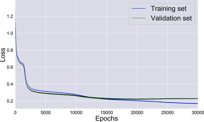
Those numbers are telling, but the diagrams that follow are even more insightful. Here’s the history of the losses during training:

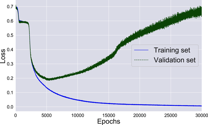
The network starts learning fast, then slows down, then accelerates again—and throughout this process, the losses on the training and the validation set decrease in lockstep. That’s until overfitting kicks in, and the two losses part ways. While the training loss keeps happily decreasing, the validation loss skyrockets. That’s an obnoxious consequence of overfitting: the longer we train this network, the worse it becomes at classifying new data.

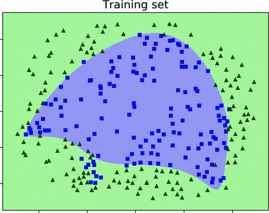
Next, let’s check out the network’s decision boundary. The following diagram shows it printed over the training set:

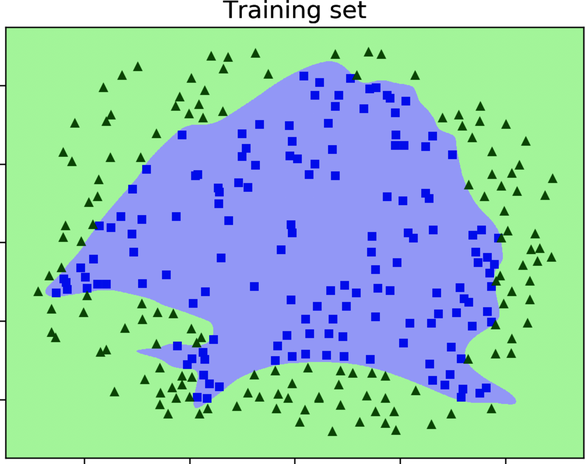
This decision boundary expertly contours the training data without missing a single point. When we overlay the boundary on the validation set, however, its limitations become apparent, as shown in this diagram:

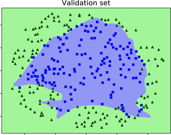
Now we see why the network is so inaccurate on the validation set. The ornate convolutions of its decision boundary do more harm than good. This boundary contours the training data closely, but it misclassifies a lot of points in the validation data. In a sense, our deep network is a victim of its own cleverness. A simpler, less baroque boundary would probably do a better job at generalizing to new data points.

We’ve seen first hand that overfitting may make a network look better, but perform worse. It’s time to smooth out that boundary, and improve the neural network’s accuracy.

L1 and L2 Regularization

L1 and L2 are two of the most common methods to regularize a decision boundary—the technical name for the operation that we informally called “smoothing out.” L1 and L2 work similarly, and they have mostly similar effects. Once you get into advanced ML territory, you may want to look deeper into their relative merits—but for our purposes in this book, I suggest you follow a simple rule: either pick randomly between L1 and L2, or try both and see which one works better.

Let’s see how L1 and L2 work.

How L1 and L2 Work

L1 and L2 rely on the same idea: add a regularization term to the neural network’s loss. For example, here’s the loss augmented by L1 regularization:

In the case of our neural network, the non-regularized loss is the cross-entropy loss. To that original loss, L1 adds the sum of the absolute values of all the weights in the network, multiplied by a constant called “lambda” (or in symbols).

Lambda is a new hyperparameter that we can use to tune the amount of regularization in the network. The greater lambda, the higher the impact of the regularization term. If lambda is 0, then the entire regularization term becomes 0, and we fall back to a non-regularized neural network.

To understand what the regularization term does to the network, remember that the entire point of training is to minimize the loss. Now that we added that term, the absolute value of the weights has become part of the loss. That means that the gradient descent algorithm will automatically try to keep the weights small, so that the loss can also stay small.

What do small weights have to do with regularization? To answer that question, consider what the weights do: the values in the first layer of the network are multiplied by some of the weights, and then combined together. That process happens again in the second layer, in the third layer, and so on, until the last layer. By consequence, if the weights are big, then a small change of the inputs tends to result in a large change of the outputs. Conversely, if the weights are small, then a small change in the inputs tends to result in a small change of the outputs. In other words, small weights cause the model function to change slowly, instead of jerking up and down.

Bottom line: L1 works by keeping the weights small, and small weights have a regularizing effect on the model function. Bingo! The L2 method uses the same exact approach, with a minor difference: instead of the absolute values of the weights, it uses their squared values.

Here’s a wrap-up of L1 and L2 regularization:

• These techniques roll the weights into the neural network’s loss.
• To minimize the loss, GD tends to keeps the weights small.
• Smaller weights tend to result in a smoother model.

Let’s try one of these techniques in our testbed neural network.

L1 in Action

Most ML libraries come with ready-to-use L1 and L2 regularization. We have to pick one, so let’s go with L1 regularization. To use L1 in our Keras neural network, we need a new import:

​	​from​ ​keras.regularizers​ ​import​ l1

Then we add a new parameter to the network’s inner layers:

17_overfitting/network_regularized.py

​	model = Sequential()
»	model.add(Dense(100, activation=​'sigmoid'​, activity_regularizer=l1(0.0004)))
»	model.add(Dense(30, activation=​'sigmoid'​, activity_regularizer=l1(0.0004)))
​	model.add(Dense(2, activation=​'softmax'​))

Keras allows you to set up L1 for each layer independently. After a few experiments, I regularized both inner layers with , which seems to strike a good balance between overfitting and underfitting. If we wanted to squeeze every last drop of accuracy out of the network, we could tune each layer’s lambda separately.

Remember that the non-regularized network gave us about 100% accuracy on the training set, and about 90% on the validation set. By contrast, here’s a run of the regularized network:

​	loss: 0.1684 - acc: 0.9509 - val_loss: 0.2278 - val_acc: 0.9263

The network’s accuracy on the validation set increased from 90% to well above 92%—which means about one fourth fewer errors. That’s pretty good! We gave up a 5% of cheap training accuracy for an extra 2% of that precious validation accuracy.

Not only is this network better than the earlier, non-regularized version—it’s also better than its shallow counterpart from the previous chapter, that was stuck around 90%. Thanks to regularization, we finally reaped the benefit of having a four-layers network instead of a three-layered network. All this talking about deep learning is starting to win us some concrete progress.

The reason for the neural network’s increased performance becomes clear if you look at its decision boundary, shown in the diagrams.

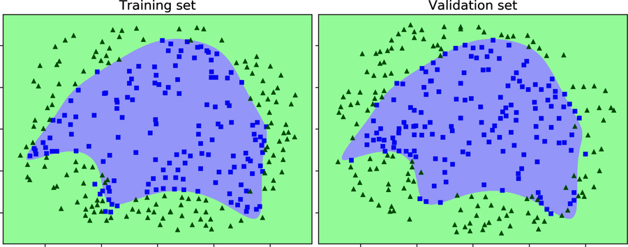
That’s a very smooth echidna. This regularized boundary isn’t as cleverly convoluted as the one we had before—but it’s all the better for that. It doesn’t fit the training data quite as well, but it’s a better fit for the validation data.

Finally, this graph shows the history of the training loss and the validation loss:

The two losses stay much closer together than before, which means that there is very little overfitting going on.

Too Much of a Good Thing

Can’t we push lambda higher and decrease overfitting even more? We might, but then we could fall out of the frying pan of overfitting and into the fire of underfitting. For example, here is what I got when I bumped up the lambda of the first hidden layer fivefold, from 0.0004 to 0.002:

​	loss: 0.2392 - acc: 0.9123 - val_loss: 0.2486 - val_acc: 0.9053

Our network’s accuracy slided back to 90%—no better than it was without regularization, and as much as a shallow, three-layered neural network. This time, however, the accuracy on the training set took a hit as well. That’s a hint that we’re now underfitting, not overfitting, the training data.

Take a look at the network’s decision boundary, and you’ll see where that loss of accuracy comes from:

See? A smoother decision boundary is all well and good, but if you overdo it, the network will lose much of its ability to shape the boundary, and it will underfit the data. That lambda of 0.0004 seems like a good trade-off between overfitting and underfitting for this network and dataset.

With that, we’re done talking about L1 and L2 regularization. However, these are far from the only regularization methods we have at our disposal. Let’s review a few more before wrapping up this chapter.