The Building Blocks of CNNs

We’ll spend the next few pages browsing through the core components of convolutional neural networks. To be clear, you shouldn’t expect that you’ll be able to build a CNN after reading through these few pages. However, you will get an idea of how they work—enough of it to run a convolutional network on CIFAR-10.

Let’s start with the most important difference between a fully connected neural network and a convolutional neural network: how they look at data.

An Image Is an Image

The first time we built a network to process images (in Chapter 6, ​Getting Real​), we noted a potentially surprising detail: the neural network doesn’t know that the examples are images. Instead, it sees them as flat sequences of bytes. We even got into the habit of flattening the images right after loading them, and we still did that just a few pages ago:

19_beyond/cifar10_fully_connected.py

​	(X_train_raw, Y_train_raw), (X_test_raw, Y_test_raw) = cifar10.load_data()
​	X_train = X_train_raw.reshape(X_train_raw.shape[0], -1) / 255

Besides rescaling the input data, this code flattens each example to a row of bytes. CIFAR-10 contains 60,000 training images, each 32 by 32 pixels per color channel, for a total of 3,072 pixels. This code reshapes the training data into a (60000, 3072) matrix. Our network flattens the test and the validation set in the same way.

By contrast, here is the equivalent code for a CNN:

​	(X_train_raw, Y_train_raw), (X_test_raw, Y_test_raw) = cifar10.load_data()
​	X_train = X_train_raw / 255

This code still loads and rescales data, but it doesn’t flatten the images. The CNN knows that it’s dealing with images, and it preserves their shape in a (60000, 32, 32, 3) tensor—60,000 images, each 32 by 32 pixels, with 3 color channels. The test and validation set would also be four-dimensional tensors.

To recap, while a fully connected network ignores the geometric information in an image, a convolutional network keeps that information around. That difference doesn’t stop at the input layer. The hidden convolutional layers in a CNN also take four-dimensional data as their input, and they output four-dimensional data for the following layer.

Speaking of convolutional layers, let’s talk about the operation they’re based on.

Convolutions

In the field of image processing, a convolution is an operation that involves two matrices: an image and a filter. Here is an example:

In this case, the filter is a (3, 3) matrix. When you convolve the image with the filter, you get a result like the one shown on the right. This specific filter highlights horizontal edges in the image—but a filter will give very different results depending on the numbers it contains.

In practice, convolutions work by sliding the filter over the image. For each position of the filters, it calculates the matrix multiplication of the overlapped section of the image with the filter. The outputs of those multiplications are assembled together to become the filter’s output. That process is easier to grasp if you visualize it. Check out the diagram that follows:

Check out “Convolutional Neural Networks in Plain English” on ProgML.

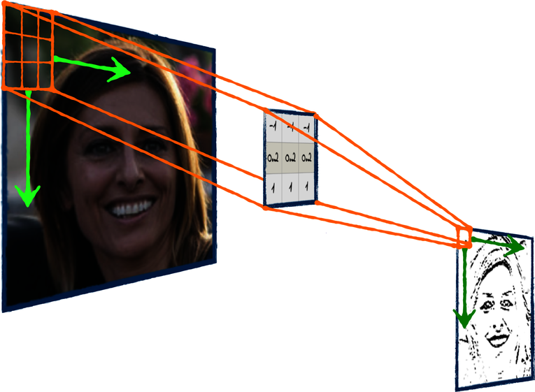
See? As the filter slides over the image, it progressively generates the output. That’s the intuition behind it, and in this book I’ll leave it at that. If you’re curious about the technical details of convolutions, you’ll find them on the ProgML^[28] site. In here, it’s enough that you know this core difference between fully connected networks and CNNs: in a fully connected network, the weights are multiplied by the input, and that is it. By contrast, in a CNN the weights are arranged in a filter that slides over the input, calculating the output piece by piece. That’s a crucial difference, as you can read in CNNs’ Secret Sauce.

CNNs' Secret Sauce

CNNs can get complicated, but the core idea behind them is simple: instead of multiplying an input by a set of weights, like fully connected networks do, slide the weights over the input, calculating the output piecemeal. When it comes to recognizing images, that trick can make a huge difference. Here is why.

Imagine that you’re building a system that recognizes human faces in pictures. To recognize a face, you must be able to recognize the peculiar shapes that a face is made of. In particular, you want to look for eyes, a nose, and other quintessentially face-y features. In practice, however, that simple notion hits a brick wall when you consider that those features might be anywhere in the image. A nose might be dead center, but it might also be tucked up in the corner of an image.

The MNIST classifiers that we built in this book work fine on images that have been carefully centered—but they’d be easily defeated if we showed them the same digits translated to different positions in a larger image. By contrast, a CNN slides its weights all over the image, like a victorian detective scanning for clues with a magnifying glass. If the digit is there, the magnifying glass will eventually pick it up, whatever its position. The same would happen with face recognition: a CNN has a chance to identify a face’s defining features, no matter where they are exactly in the picture. That property is called translation invariance, and it’s the secret sauce that allows CNNs to recognize images.

 

I just mentioned how a convolutional layer applies a filter to its inputs—but in reality, it doesn’t need to be only one filter. In general, a convolutional layer applies multiple filters at once. The diagram shows a stack of filters applied to an image, resulting in a stack of outputs.

As usual when you work with neural networks, it’s easy to get confused by the dimensions of all the matrices and tensors involved. (In case you don’t remember, a “tensor” is like a matrix, but it can have more than two dimensions.) Let’s check out the dimensions of the tensors in this example. Let’s say the image is 100 pixels wide and 100 pixels high with 3 color channels—a (100, 100, 3) tensor. If each filter is a square of 5 by 5 numbers, and we have 6 filters, then the stack of filters is a (5, 5, 6) tensor. Based on those inputs, let’s calculate the dimensions of the output tensor.

There are multiple parameters to a convolution, and they can result in a tensor with different dimensions. In this book, however, we’ll only use the default values of those parameters. For the default case, we can calculate the dimensions of the output like this:

• The height of the output is the height of the input, minus the height of the filter, plus 1. In our case, that’s 100 - 5 + 1 = 96

• The same rule applies to the width of the output, so that would also be 96.

• Each filter outputs one matrix, so the depth of the output tensor is equal to the number of filters.

Here’s the convolution again, with the dimensions of all the tensors involved:

So now you have an idea of what a convolution looks like and how to calculate the dimensions of its result. Let’s see how convolutions are used in a neural network.

Convolutional Layers

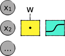
Remember how a fully connected layer works—it’s a matrix multiplication between the inputs and the weights, followed by an activation function, as shown in the diagram that follows:

Now arrange the weights into a stack of filters, replace that matrix multiplication with a convolution (that is sometimes denoted by an asterisk), and boom! You get a convolutional layer, as shown in the next diagram:

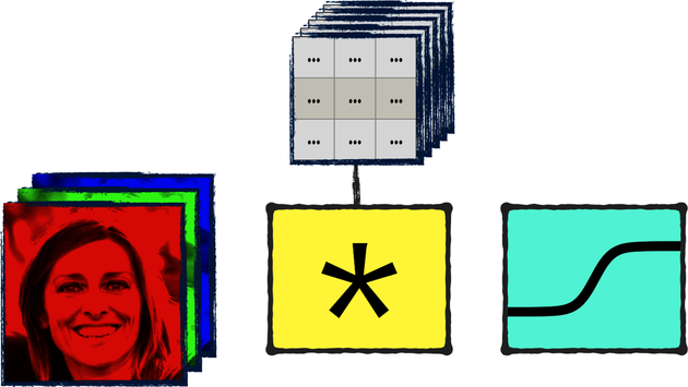
Note that both these diagrams are simplifications, because they show the input as a single image. In truth, a neural network generally processes multiple images at once, and the number of images adds another dimension to the input. So the input to a fully connected layer has not one, but two dimensions; the input to a convolutional layer has not three, but four dimensions. In both cases, we skip the first dimensions when we visualize the neural networks to avoid cluttering the diagrams.

Enough diagrams; let’s see some code. Here is how you add a convolutional layer to a Keras model:

​	model.add(Conv2D(16, (3, 3), activation=​'relu'​))

All the numbers in the preceding line are arbitrarily chosen hyperparameters that you can tune, and you’ll get a chance to do so at the end of this chapter. This specific convolutional layer has 16 filters, and each filter is a 3 by 3 square. Keras takes care of initializing the values in the filters, just like it does for the weights of a fully connected network. As usual, the activation is the layer’s activation function—in this case, a ReLU.

Now you know what a single convolutional layer looks like. Let’s put a few of those layers together and build our own CNN.

Convolutions Can Get Complicated

As I talk about convolutions, I’m making a lot of implicit assumptions. First of all, I’m assuming that our convolutions operate on images. To process images, you need bi-dimensional convolutions called Conv2D in Keras. Different kinds of data might require higher-dimensional convolutions. For example, video has the additional dimension of time, and it could be processed with three-dimensional convolutions.

Even if you stick with bi-dimensional convolutions, there are more parameters to a convolution that just the filters. For example, a parameter named padding adds an empty frame around the input image to control the dimensions of the output.

If you decide to delve deeper into CNN, you’ll take a long hard look at those variations on the main theme. In this book, we’ll limit ourselves to run-of-the-mill convolutions.