9. Graphs
In this chapter we explain how to plot graphs in MATLAB. Both two-dimensional and three-dimensional graphs are presented. A graph in MATLAB appears in its own window (not on the command line). First, we will consider two-dimensional or planar graphs. To plot a two-dimensional graph, we need two vectors. Here is a simple example using two vectors x and y along with the MATLAB command plot:
>> x = [1 2 3 4 5]
x =
1 2 3 4 5
>> y = [3 9 12 10 6]
y =
3 9 12 10 6
>> plot(x,y)
The resulting graph is displayed in its own window and is shown in Figure 9.1. Note how the command plot was used above along with the two vectors x and y. This is the simplest use of this command in MATLAB.
We can add some information to the above graph using other MATLAB commands that are associated with the plot command. For example, we can use the title command to add a title to the graph. Also, we can use the MATLAB commands xlabel and ylabel to add labels to the x-axis and the y-axis. But before using these three commands (title, xlabel, ylabel), we need to keep the plotted graph in its window. For this we use the hold on command as follows:
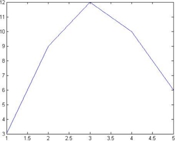
Figure 9.1: A simple use of the plot command
>> hold on
>> title('This is an example of a simple graph')
>> xlabel('x')
>> ylabel('y')
After executing the above commands, the plotted graph appears as shown in Figure 9.2 with the title and axes labels clearly displayed.
Let us now plot the mathematical function y = x2 – 4 in the range x from -3 to +3. First, we need to define the vector x, then calculate the vector y using the above formula. Then we use the plot command as usual for the two vectors x and y. Finally, we use the other commands to display the title and axis label information on the graph.
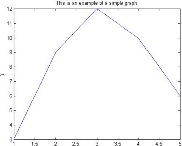
Figure 9.2: Title and axis information displayed on graph
The following are the needed commands. The resulting graph is shown in Figure 9.3.
>> x = [-3 -2 -1 0 1 2 3]
x =
-3 -2 -1 0 1 2 3
>> y = x.^2 -3
y =
6 1 -2 -3 -2 1 6
>> plot(x,y)
>> hold on
>> title('This is another example of the plot command')
>> xlabel('x-axis')
>> ylabel('y-axis')
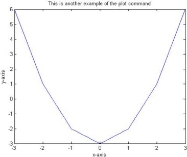
Figure 9.3: Example of plotting a mathematical function
It is seen from the above graphs that they are plotted with solid lines. The line style may be changed from solid to dotted, dashed, or dash-dot lines by changing the parameters in the plot command. Use the command plot(x,y,’:’) to get a dotted line, the command plot(x,y,’--‘) to get a dashed line, the command plot(x,y,’-.’) to get a dash-dot line, and the default command plot(x,y,’-‘) to get a solid line.
In addition, the color of the plotted line may be changed. Use the command plot(x,y,’b’) to get a blue line. Replace the b with g for green, r for red, c for cyan, m for magnetta, y for yellow, k for black, and w for white. Consult the MATLAB manual for a full list of the color options. Note that colors are not displayed in this book.
In addition to changing the line style and color, we can include symbols at the plotted points. For example, we can use the circle or cross symbols to denote the plotted points. Use the command plot(x,y,’o’) to get a circle symbol. Replace the o with x to get a cross symbol, + for a plus sign symbol, * for a star symbol, s for a square symbol, d for a diamond symbol, and . for a point symbol. There are other commands for other symbols like different variations of triangles, etc. Again, consult the MATLAB manual for the full list of available symbols.
The above options for line style, color, and symbols can be combined in the same command. For example use the command plot(x,y,’rx:’) to get a red dotted line with cross symbols. Here is the previous example with a red dotted line with cross symbols but without the title and label information (note that no colors appear in this book). See Figure 9.4 for the resulting graph.
>> plot(x,y,'rx:')
Next, consider the following example where we show another use of the plot command. In this example, we plot two curves on the same graph. We use the modified plot command as plot(x,y,x,z) to plot the two curves. MATLAB plots the two mathematical functions y and z (on the y-axis) as a function of x (on the x-axis). We also use the MATLAB command grid to show a grid on the plot. Here are the needed commands34. The resulting graph is shown in Figure 9.5.
>> x = 0:pi/20:2*pi;
>> y = sin(x);
>> z = cos(x);
>> plot(x,y,'-',x,z,'--')
>> hold on;
>> grid on;
>> title('Sine and Cosine Functions')
>> xlabel('x-axis')
>> ylabel('sine and cosine')
>> legend('sinx','cosx')
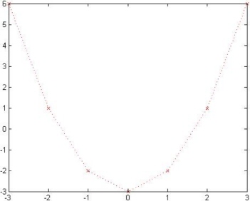
Figure 9.4: A red dotted line with cross symbols
Note in the above example that we used semicolons to suppress the output. Also, note the use of the MATLAB command legend to get a legend displayed at the top right corner of the graph. We can further use several axis commands to customize the appearance of the two axes including the tick marks, but this is beyond the scope of this book. Consult the MATLAB manual for further details about these commands.
There are some interactive plotting tools available in MATLAB to further customize the resulting graph. These tools are available from the menus of the graph window – the window where the graph appears.
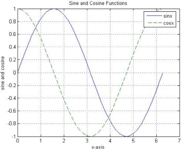
Figure 9.5: Example of two curves on the same graph
There are other specialized plots35 that can be drawn automatically by MATLAB. For example, there are numerous plots that are used in statistics that can be generated by MATLAB. In particular, a pie chart can be generated by using the MATLAB command pie, a histogram can be generated by using the MATLAB command hist, and a rose diagram can be generated by using the MATLAB command rose. In addition, graphs of curves with polar coordinates can be generated by using the MATLAB command polar.
Our final two-dimensional graph will feature the use of the MATLAB command subplot. The use of this command will enable you to present several plot diagrams on the same graph. In this example, we use four instances of the subplot command to show four diagrams on the same plot. We will plot four mathematical functions – each on its own diagram – but the four diagrams will appear on the same graph. We can do this by playing with the parameters of the subplot command. Note that the diagrams are shown without title or axis labels in order to emphasize the use of the subplot command. Here are the necessary MATLAB commands36 used with semicolons to suppress the output:
>> x = [ 1 2 3 4 5 6 7 8 9 10];
>> y = x.^2;
>> z = sqrt(x);
>> w = 2*x - 3;
>> v = x.^3;
>> subplot(2,2,1)
>> hold on;
>> plot(x,y)
>> subplot(2,2,2)
>> plot(x,z)
>> subplot(2,2,3)
>> plot(x,w)
>> subplot(2,2,4)
>> plot(x,v)
Note the use of the three parameters of the subplot command. The first two parameters (2,2) indicate that the graph area should be divided into four quadrants with each row and column comprising of two sub-areas for plots. The third parameter indicates in which sub-area the next plot will appear. Note also that each subplot command is followed by a corresponding plot command. Actually, each subplot command reserves a specific area for the plot while the subsequent corresponding plot command does the actual plotting. The resulting graph is shown in Figure 9.6. You can control the number and arrangement of the diagrams that are displayed by controlling the three parameters of the subplot command.
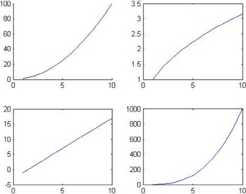
Figure 9.6: Use of the MATLAB command subplot
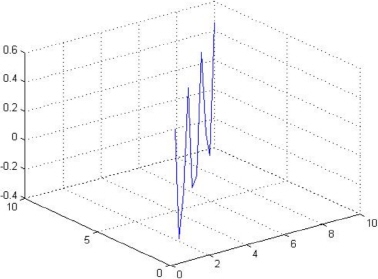
Next, we will discuss how to generate three-dimensional graphs with MATLAB. There are mainly four commands that can be used in MATLAB for plotting three-dimensional graphs. The first command is plot3 which is used to plot curves in space. It requires three vectors as input. Here is an example of this command followed by the resulting graph as shown in Figure 9.7.
>> x = [1 2 3 4 5 6 7 8 9 10]
x =
1 2 3 4 5 6 7 8 9 10
>> y = [1 2 3 4 5 6 7 8 9 10]
y =
1 2 3 4 5 6 7 8 9 10
>> z = sin(x).*cos(y)
z =
Columns 1 through 6
0.4546 -0.3784 -0.1397 0.4947 -0.2720 -0.2683
Columns 7 through 10
0.4953 -0.1440 -0.3755 0.4565
>> plot3(x,y,z)
>> hold on;
>> grid on;
It should be noted that the title, xlabel, and ylabel commands can also be used with three-dimensional graphs. For the z-axis, the MATLAB command zlabel is also used in a way similar to the xlabel and ylabel commands.
The second command in MATLAB for three dimensional plots is mesh. The use of the mesh command is used to generate mesh surfaces. The simplest use of this command is with a matrix. It assumes that the matrix elements are values of a grid spanning the matrix dimensions. The values of the elements of the matrix are taken automatically along the z-axis while the numbers of rows and columns are taken along the x- and y-axes. Here is an example followed by the resulting graph as shown in Figure 9.8.
>> A = [10 14 20 37 5 17 11 ; 12 20 40 20 11 5 14 ; 30 51 12 17 20 30 2 ; 24 34 56 10 14 5 40 ; 34 12 33 12 26 10 15 ; 12 45 13 23 35 10 7 ; 10 20 13 34 32 10 7]
A =
10 14 20 37 5 17 11
12 20 40 20 11 5 14
30 51 12 17 20 30 2
24 34 56 10 14 5 40
34 12 33 12 26 10 15
12 45 13 23 35 10 7
10 20 13 34 32 10 7
>> mesh(A)
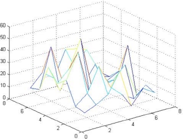
Figure 9.8: Use of the mesh command
If a matrix or a grid is not available, then a grid can be generated using the MATLAB command meshgrid but this is beyond the scope of this book. Again, the reader should use the title and axis information commands to display information on the graph but these are not shown in this example.
The third MATLAB command for three-dimensional plots is the surf command. Its use is similar to the mesh command. Here is an example of its use with the same matrix A of the previous example followed by the resulting graph as shown in Figure 9.9.
>> surf(A)
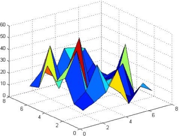
Figure 9.9: Use of the surf command
The above three-dimensional plot is usually shown in color in MATLAB but we are not able to display colors in this book. Again, the MATLAB command meshgrid may be used to generate a grid for the three-dimensional plot if one is not available. Again, the reader should use the title and axis information commands to display these types of information on the plot above but these are not used in this example.
The fourth command for three-dimensional plots is the MATLAB command contour. The use of this command produces contour plots of three-dimensional surfaces. The use of this command is similar to the mesh and surf commands. Here is an example of its use with the same matrix A that was used previously followed by the resulting graph as shown in Figure 9.10.
>> contour(A)
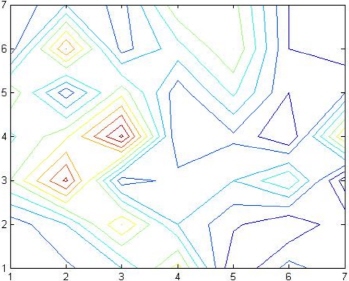
Figure 9.10: Use of the contour command
The above contour plot is usually shown in color in MATLAB but we are not able to display colors in this book. Again, the MATLAB command meshgrid may be used to generate a grid for the contour plot if one is not available. The reader can add the contour heights to the graph using the MATLAB command clabel.
There are some variations of the mesh and surf commands in MATLAB. For example, the meshc and surfc commands produce the same mesh and surface plots as the commands mesh and surf but with the contour plot appearing underneath the surface. Here is an example of the use of the surfc command with the same matrix A used previously followed by the resulting graph as shown in Figure 9.11.
>> surfc(A)
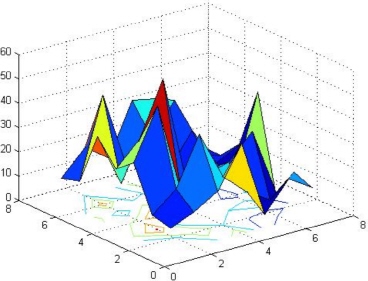
Figure 9.11: Use of the surfc command
Another variation is the meshz command which produces the same three-dimensional plot as the mesh command but with a zero plane underneath the surface. The use of this command is very simple and is not shown here.
In the next chapter, we discuss solution of equations in MATLAB.
Exercises
Solve all the exercises using MATLAB. All the needed MATLAB commands for these exercises were presented in this chapter.
- Plot a two-dimensional graph of the two vectors
x= [1 2 3 4 5 6 7] andy= [10 15 23 43 30 10 12] using theplotcommand. - In Exercise 1 above, add to the graph a suitable title along with labels for the x-axis and the y-axis.
- Plot the mathematical function y = 2x3 + 5 in the range
xfrom-6to+6. Include a title for the graph as well as labels for the two axes. - Repeat the plot of Exercise 3 above but show the curve with a blue dashed line with circle symbols at the plotted points.
- Plot the two mathematical functions
 and
and  such that the two curves appear on the same diagram. Make the range for
 xbetween0and 3π with increments of . Distinguish the two curves by plotting one with a dashed line and the other one with a dotted line. Include the title and axis information on the graph as well as a grid and a legend.
 - Plot the following four mathematical functions each with its own diagram using the
subplotcommand. The functions are y = 2x3 − 4, z = x + 1, , and v = x2 + 3. Use the vector
 x= [1 2 3 4 5 6 7 8 9 10] as the range forx. There is no need to show title or axis information. - Use the
plot3command to show a three-dimensional curve of the equation z = 2sin(xy) . Use the vectorx= [1 2 3 4 5 6 7 8 9 10] for bothxandy. There is no need to show title or axis information. - Use the
meshcommand to plot a three-dimensional mesh surface of elements of the matrixMgiven below. There is no need to show title or axis information.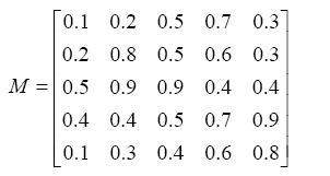
- Use the
surfcommand to plot a three-dimensional surface of the elements of the matrixMgiven in Exercise 8 above. There is no need to show title or axis information. - Use the
contourcommand to plot a contour map of the elements of the matrixMgiven in Exercise 8 above. There is no need to show the contour values on the graph. - Use the
surfccommand to plot a three-dimensional surface along with contours underneath it of the matrixMgiven in Exercise 8 above. There is no need to show title or axis information.