Solutions to Exercises
1. Introduction
- Perform the operation 3*4+6. The order of the operations will be discussed in subsequent chapters.
>> 3*4+6
ans =
18 - Perform the operation cos(5). The value of
5is in radians.>> cos (5)
ans =
0.2837 - Perform the operation
 for x = 4.
>> x = 4
x =
4
>> 3*sqrt(6+x)
ans =
9.4868 - Assign the value of 5.2 to the variable y.
- Assign the values of 3 and 4 to the variables x and y, respectively, then calculate the value of z where z = 2x − 7y.
>> x = 3;
>> y = 4;
>> z = 2*x - 7*y
z =
-22 - Obtain help on the inv command.
>> help inv
INV Matrix inverse.
INV(X) is the inverse of the square matrix X.
A warning message is printed if X is badly scaled or nearly singular.
See also slash, pinv, cond, condest, lsqnonneg, lscov.
Overloaded functions or methods (ones with the same name in other directories) help sym/inv.m
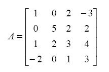
Reference page in Help browser doc inv - Generate the following matrix: A
>> A = [1 0 2 -3 ; 0 5 2 2 ; 1 2 3 4 ; -2 0 1 3]
A =
1 0 2 -3
0 5 2 2
1 2 3 4
-2 0 1 3 - Generate the following vector b
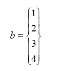
>> b = [1 ; 2 ; 3 ; 4]
b =
1
2
3
4 - Evaluate the vector c where
 where A is the matrix given in Exercise 7 above and b is the vector given in Exercise 8 above.
- Solve the following system of simultaneous algebraic equation using Gaussian elimination.
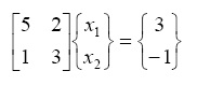
>> A = [ 5 2 ; 1 3]
A =
5 2
1 3
>> b = [3 ; −1]
b =
3
-1
>> x = A\b
x =
0.8462
-0.6154 - Solve the system of simultaneous algebraic equations of Exercise 10 above using matrix inversion.
- Generate the following matrix X:
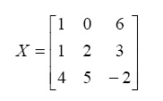
>> X = [1 0 6 ; 1 2 3 ; 4 5 -2]
X =
1 0 6
1 2 3
4 5 -2 - Extract the sub-matrix in rows 2 to 3 and columns 1 to 2 of the matrix X in Exercise 12 above.
>> X(2:3,1:2)
ans =
1 2
4 5 - Extract the second column of the matrix X in Exercise 12 above.
>> X(1:3,2)
ans =
0
2
5 - Extract the first row of the matrix X in Exercise 12 above.
>> X(1,1:3)
ans =
1 0 6 - Extract the element in row 1 and column 3 of the matrix X in Exercise 12 above.
>> X(1,3)
ans =
6 - Generate the row vector x with integer values ranging from 1 to 9.
>> x = [1 2 3 4 5 6 7 8 9]
x =
1 2 3 4 5 6 7 8 9 - Plot the graph of the function y = x3 − 2 for the range of the values of x in Exercise 17 above.
>> y = x.^3 - 2
y =
-1 6 25 62 123 214 341 510 727
>> plot(x,y)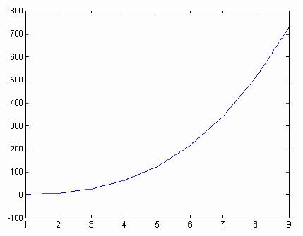
- Generate a 4 x 4 magic square. What is the total of each row, column, and diagonal in this matrix.
>> magic(4)
ans =
16 2 3 13
5 11 10 8
9 7 6 12
4 14 15 1The sum of each row, column, or diagonal is 34.
2. Arithmetic Operations
- Perform the addition operation 7+9.
- Perform the subtraction operation 16-10.
>> 16−10
ans =
6 - Perform the multiplication operation 2*9.
>> 2*9
ans =
18 - Perform the division operation 12/3.
>> 12/3
ans =
4 - Perform the division operation 12/5.
>> 12/5
ans =
2.4000 - Perform the exponentiation operation 3^5.
- Perform the exponentiation operation 3*(-5).
>> 3^(-5)
ans =
0.0041 - Perform the exponentiation operation (-3)^5.
>> (−3)^5
ans =
−243 - Perform the exponentiation operation -3^5.
>> −3^5
ans =
−243 - Compute the value of

>> 2*pi/3
ans =
2.0944 - Obtain the value of the smallest number that can be handled by MATLAB.
- Perform the multiple operations 5+7-15.
>> 5+7-15
ans =
-3 - Perform the multiple operations (6*7)+4.
>> 6*7 +4
ans =
46 - Perform the multiple operations 6*(7+4).
>> 6*(7+4)
ans =
66 - Perform the multiple operations 4.5 + (15/2).
>> 4.5 + 15/2
ans =
12 - Perform the multiple operations (4.5 + 15)/2.
- Perform the multiple operations (15 – 4 + 12)/5 – 2*(7^4)/100.
>> (15–4+12) /5 – 2*(7^4)/100
ans =
-43.4200 - Perform the multiple operations (15 – 4) + 12/5 – (2*7)^4/100.
>> (15–4) + 12/5 – (2*7)^4/100
ans =
−370.7600 - Define the number 2/3 as a symbolic number.
>> sym(2/3)
ans =
2/3 - Perform the fraction addition (2/3) + (3/4) numerically.
>> 2/3 + 3/4
ans =
1.4167 - Perform the fraction addition (2/3) + (3/4) symbolically.
3. Variables
- Perform the operation 2*3+7 and store the result in the variable
w.>> 2*3+7
ans =
13 - Define the three variables
a, b, andcequal to4, −10, and3.2, respectively.>> a = 4
a =
4
>> b = −10
b =
−10
>> c = 3.2
c =
3.2000 - Define the two variables
yandYequal to10and100. Are the two variables identical?>> y = 10
y =
10
>> Y = 100
Y =
100The two variables are not identical.
- Let
x=5.5andy=−2.6. Calculate the value of the variablez = 2x−3y.x =
5.5000
>> y = −2.6
y =
−2.6000
>> z = 2*x − 3*y
z =
18.8000 - In Exercise 4 above, calculate the value of the variable
w=3y−z + x/y. - Let
r=6.3ands = 5.8. Calculate the value of the variablefinaldefined byfinal=r + s - r*s.>> r = 6.3
r =
6.3000
>> s = 5.8
s =
5.8000
>> final = r + s - r*s
final =
-24.4400 - In Exercise 6 above, calculate the value of the variable
this_is_the_resultdefined bythis_is_the_result = r^2 – s^2.>> this_is_the_result = r^2 − s^2
this_is_the_result =
6.0500 - Define the three variable
width, Width, andWIDTHequal to 1.5, 2.0, and 4.5, respectively. Are these three variables identical?The three variables are not identical.
- Write the following comment in MATLAB:
This line will not be executed.% This line will not be executed.
- Assign the value of
3.5to the variablesthen add a comment about this assignment on the same line.>> s = 3.5 % the variable s is assigned the value 3.5
s =
3.5000 - Define the values of the variables
y1andy2equal to7and9then perform the calculationy3 = y1 – y2/3. (Note: 2 in the formula is a subscript and should not be divided by 3). - Perform the operation
2*m – 5. Do you get an error? Why?>> 2*m − 5
??? Undefined function or variable 'm'.We get an error message because the variable
mis not defined. - Define the variables
costandprofitequal to175and25, respectively, then calculate the variablesale_pricedefined bysale_price=cost + profit. - Define the variable
centigradeequal to28then calculate the variablefahrenheitdefined byfahrenheit = (centigrade*9/5) + 32.>> centigrade = 28
centigrade =
28
>> fahrenheit = (centigrade*9/5) + 32
fahrenheit =
82.4000 - Use the
format shortandformat longcommands to write the values of14/9to four decimals and sixteen digits, respectively.>> format long
>> 14/9
ans =
1.55555555555556
>> format short
>> 14/9
ans =
1.5556 -
Perform the
whocommand to get a list of the variables stored in this session.
>> who
Your variables are:WIDTH fahrenheit x
Width final y
Y profit y1
a r y2
ans s y3
b sale_price z
c this_is_the_result centigrade
w cost width
- Perform the
whoscommand to get a list of the variables stored in this session along with their details.
>> whos
- Clear all the variables stored in this session by using the
clearcommand.>> clear
>> - Calculate both the area and perimeter of a rectangle of sides 5 and 7. No units are used in this exercise.
a =
5
>> b = 7
b =
7
>> area = a*b
area =
35
>> perimeter = 2*(a+b)
perimeter =
24 -
Calculate both the area and perimeter of a circle of radius 6.45. No units are used in this exercise.
>> r = 6.45
r =
6.4500
>> area = pi*r^2
area =
130.6981
>> perimeter = 2*pi*r
perimeter =
40.5265 - Define the symbolic variables x and z with values 4/5 and 14/17.
- In Exercise 21 above, calculate symbolically the value of the symbolic variable y defined by y = 2x – z.
>> y = sym(2*x − z)
y =
66/85 - Calculate symbolically the area of a circle of radius 2/3 without obtaining a numerical value. No units are used in this exercise.
>> radius1 = 2/3
radius1 =
0.6667
>> radius1 = sym(radius1)
radius1 =
2/3
>> area = pi*radius1^2
area =
4/9*pi -
Calculate symbolically the volume of a sphere of radius 2/3 without obtaining a numerical value. No units are used in this exercise.
>> radius2 = 2/3
radius2 =
0.6667
>> radius2 = sym(radius2)
radius2 =
2/3
>> volume = (4/3)*pi*radius2^3
volume =
32/81*pi - In Exercise 23 above, use the
doublecommand to obtain the numerical value of the answer.>> double(area)
ans =
1.3963 - In Exercise 24 above, use the
doublecommand to obtain the numerical value of the answer.>> double(volume)
ans =
1.2411 -
Define the symbolic variables
yanddatewithout assigning any numerical values to them.>> y = sym('y')
y =
y
>> date = sym('date')
date =
date
4. Mathematical Functions
- Compute the square root of 10.
>> sqrt(10)
ans =
3.1623 - Compute the factorial of 7.
>> factorial(7)
ans =
5040 - Compute the cosine of the angle 45 where 45 is in radians.
- Compute the cosine of the angle 45 where 45 is in degrees.
>> cos(45*pi/180)
ans =
0.7071 - Compute the sine of the angle of 45 where 45 is in degrees.
>> sin(45*pi/180)
ans =
0.7071 - Compute the tangent of the angle 45 where 45 is in degrees.
>> tan(45*pi/180)
ans =
1.0000 - Compute the inverse tangent of 1.5.
>> atan(1.5)
ans =
0.9828The above result is in radians.
- Compute the tangent of the angle
 . Do you get an error? Why?
We get a very large number approaching infinity because the tanget function is not define at
. - Compute the value of exponential function e3.
>> exp(3)
ans =
20.0855 - Compute the value of the natural logarithm ln 3.5.
>> log(3.5)
ans =
1.2528 - Compute the value of the logarithm log10 3.5.
>> log10(3.5)
ans =
0.5441 - Use the MATLAB rounding function
roundto round the value of 2.43. - Use the MATLAB remainder function
remto obtain the remainder when dividing 5 by 4.>> rem(5,4)
ans =
1 - Compute the absolute value of -3.6.
>> abs(-3.6)
ans =
3.6000 - Compute the value of the expression

>> 1.5 - 2*sqrt(6.7/5)
ans =
-0.8152 - Compute the value of sin 2 π + cos2 π.
>> sin(pi)^2 + cos(pi)^2
ans =
1 - Compute the value of log10 0. Do you get an error? Why?
We get minus infinity because the logarithmic function is not defined at zero.
- Let
 and y = 2π. Compute the value of the expression 2sin x cos y.
>> x = 3*pi/2
x =
4.7124
>> y = 2*pi
y =
6.2832
>> 2*sin(x)*cos(y)
ans =
-2 - Compute the value of
 symbolically and simplify the result.
- Compute the value of numerically.
>> double(ans)
ans =
6.7082 - Compute the sine of the angle 45 (degrees) symbolically.
>> sym(sin(45*pi/180))
ans =
sqrt(1/2) - Compute the cosine of the angle 45 (degrees) symbolically.
> sym(cos(45*pi/180))
ans =
sqrt(1/2) - Compute the tangent of the angle 45 (degrees) symbolically.
- Compute the value of eπ/2 symbolically.
>> sym(exp(pi/2))
ans =
5416116035097439*2^(-50)
- Compute the value of eπ/2 numerically.
>> double(ans)
ans =
4.8105
5. Complex Numbers
- Compute the square root of -5.
>> sqrt(-5)
ans =
0 + 2.2361i - Define the complex number
 .
.
>> 4-3*sqrt(-8)
ans =
4.0000 - 8.4853i - Define the two complex numbers with variables x and y where x = 2 − 6i and y = 4 +11i.
- In Exercise 3 above, perform the addition and subtraction operations x + y and x − y.
>> x+y
ans =
6.0000 + 5.0000i
>> x-y
ans =
-2.0000 -17.0000i - In Exercise 3 above, perform the multiplication and division operations x y and

- In Exercise 3 above, perform the exponentiation operations x4 and y -3.
>> x^4
ans =
4.4800e+002 +1.5360e+003i
>> y^(-3)
ans =
-5.3979e-004 +3.1229e-004i - In Exercise 3 above, perform the multiple operations 4x − 3y + 9.
>> 4*x-3*y+9
ans =
5.0000 -57.0000i - In Exercise 3 above, perform the multiple operations ix − 2y − 1.
>> i*x-2*y-1
ans =
-3.0000 -20.0000i - Compute the magnitude of the complex number 3 − 5i.
- Compute the angle of the complex number 3 − 5i in radians.
>> angle(3−5i)
ans =
-1.0304 - Compute the angle of the complex number 3 − 5i in degrees.
>> angle(3-5i)*180/pi
ans =
-59.0362 - Extract the real and imaginary parts of the complex number 3 − 5i.
>> real(3−5i)
ans =
3
>> imag(3−5i)
ans =
−5 - Obtain the complex conjugate of the complex number 3 − 5i.
- Compute the sine, cosine, and tangent functions of the complex number 3 − 5i.
>> sin(3-5i)
ans =
10.4725 +73.4606i
>> cos(3-5i)
ans =
-73.4673 +10.4716i
>> tan(3-5i)
ans =
-0.0000 - 0.9999i - Compute e3-5i and ln(3 − 5i).
>> exp(3-5i)
ans =
5.6975 +19.2605i
>> log(3-5i)
ans =
1.7632 - 1.0304i -
Compute the values of sin
 and eπi /2.
>> sin(pi*i/2)
ans =
0 + 2.3013i
>> cos(pi*i/2)
ans =
2.5092
>> exp(pi*i/2)
ans =
0.0000 + 1.0000i - Compute the value of (3 + 4i)(2-i).
>> (3+4i)^(2-i)
ans =
61.3022 +15.3369i - Obtain
 symbolically.
>> sym(sqrt(-13))
ans =
(0)+(sqrt(13))*i - Obtain the magnitude of the complex number 3− 5i symbolically.
- Obtain the angle of the complex number 3− 5i symbolically. Make sure that you use the
doublecommand at the end.>> sym(angle(3-5i))
ans =
-4640404691986088*2^(-52)
>> double(ans)
ans =
-1.0304 - Obtain the cosine function of the complex number 3− 5i symbolically. Make sure that you use the
doublecommand at the end.>> sym(cos(3-5i))
ans =
(-5169801091137321*2^(-46))+(5894962905280379*2^(-49))*i
>> double(ans)
ans =
-73.4673 +10.4716i
6. Vectors
- Store the vector [2 4 -6 0] in the variable w.
>> w = [2 4 -6 0]
w=
2 4 -6 0 - In Exercise 1 above, extract the second element of the vector w.
> w(2)
ans =
4 - In Exercise 1 above, generate the vector z where

>> z = pi*w/2
z =
3.1416 6.2832 -9.4248 0 - In Exercise 3 above, extract the fourth element of the vector z.
>> z(4)
ans =
0 - In Exercise 3 above, extract the first three elements of the vector z.
- In Exercise 3 above, find the length of the vector z.
>> length(z)
ans =
4 - In Exercise 3 above, find the total sum of the values of the elements of the vector z.
>> sum(z)
ans =
0 - In Exercise 3 above, find the minimum and maximum values of the elements of the vector z.
>> min(z)
ans =
-9.4248
>> max(z)
ans =
6.2832 - Generate a vector r with real values between 1 and 10 with an increment of 2.5.
- Generate a vector s with real values of ten numbers that are equally spaced between 1 and 100.
>> s = linspace(1,100,10)
s =
1 12 23 34 45 56 67 78 89 100 - Form a new vector by joining the two vectors [9 3 -2 5 0] and [1 2 - 4].
>> a = [9 3 -2 5 0]
a =
9 3 -2 5 0
>> b = [1 2 -4]
b =
1 2 -4
>> c = [a b]
c =
9 3 -2 5 0 1 2 -4 - Form a new vector by joining the vector [9 3 -2 5 0] with the number 4.
- Add the two vectors [0.2 1.3 -3.5] and [0.5 -2.5 1.0].
>> x = [0.2 1.3 -3.5]
x =
0.2000 1.3000 -3.5000
>> y = [0.5 -2.5 1.0]
y =
0.5000 -2.5000 1.0000
>> x+y
ans =
0.7000 -1.2000 -2.5000 - Subtract the two vectors in Exercise 13 above.
>> x-y
ans =
-0.3000 3.8000 -4.5000 - Try to multiply the two vectors in Exercise 13 above. Do you get an error message? Why?
We get an error because the two vectors do not have the same length.
- Multiply the two elements in Exercise 13 above element by element.
>> x.*y
ans =
0.1000 -3.2500 -3.5000 - Divide the two elements in Exercise 13 above element by element.
>> x./y
ans =
0.4000 -0.5200 -3.5000 - Find the dot product of the two vectors in Exercise 13 above.
>> x*y'
ans =
-6.6500 - Try to add the two vectors [1 3 5] and [3 6]. Do you get an error message? Why?
>> r = [ 1 3 5 ]
r =
1 3 5
>> s = [ 3 6 ]
s =
3 6
>> r+s
??? Error using ==> plus
Matrix dimensions must agree.We get an error message because the two vectors do not have the same length.
- Try to subtract the two vectors in Exercise 20 above. Do you get an error message? Why?
>> r-s
??? Error using ==> minus
Matrix dimensions must agree.We get an error message because the two vectors do not have the same length.
- Let the vector w be defined by w = [0.1 1.3 -2.4]. Perform the operation of scalar addition 5+w.
>> w = [0.1 1.3 -2.4]
w =
0.1000 1.3000 -2.4000
>> 5+w
ans =
5.1000 6.3000 2.6000 - In Exercise 22 above, perform the operation of scalar subtraction -2-w.
- In Exercise 22 above, perform the operation of scalar multiplication 1.5*w.
>> 1.5*w
ans =
0.1500 1.9500 -3.6000 - In Exercise 22 above, perform the operation of scalar division w/10.
>> w/10
ans =
0.0100 0.1300 -0.2400 - In Exercise 22 above, perform the operation 3 − 2*w/5.
>> 3-2*w/5
ans =
2.9600 2.4800 3.9600 - Define the vector b by b = [0 pi/3 2pi/3 pi]. Evaluate the three vectors sin b, cosb, and tan b (element by element).
- In Exercise 26 above, evaluate the vector eb (element by element).
>> exp(b)
ans =
1.0000 2.8497 8.1205 23.1407 - In Exercise 26 above, evaluate the vector
 (element by element).
>> sqrt(b)
ans =
0 1.0233 1.4472 1.7725 - Try to evaluate the vector 3b. Do you get an error message? Why?
Yes, because this operation needs to be performed element by element.
- Perform the operation in Exercise 29 above element by element?
>> 3.^b
ans =
1.0000 3.1597 9.9834 31.5443 - Generate a vector of 1’s with a length of 4 elements.
> ones(1,4)
ans =
1 1 1 1 - Generate a vector of 0’s with a length of 6 elements.
>> zeros(1,6)
ans =
0 0 0 0 0 0 - Sort the elements of the vector [0.35 -1.0 0.24 1.30 -0.03] in ascending order.
- Generate a random permutation vector with 5 elements.
>> randperm(5)
ans =
2 4 3 5 1 - For the vector [2 4 -3 0 1 5 7], determine the range, mean, and median.
- Define the symbolic vector x = [r s t u v].
>> syms r s t u v
>> x = [r s t u v]x= [ r, s, t, u, v] - In Exercise 36 above, perform the addition operation of the two vectors
xand [1 0 -2 3 5] to obtain the new symbolic vectory.>> r = [1 0 -2 3 5]
r =
1 0 -2 3 5
>> y = x+r
y =
[ r+1, s, t-2, u+3, v+5] - In Exercise 37 above, extract the third element of the vector
y.>> y(3)
ans =
t-2 - In Exercise 37 above, perform the operation
2*x/7 + 3*y.>> 2*x/7 + 3*y
ans =
[ 23/7*r+3, 23/7*s, 23/7*t-6, 23/7*u+9, 23/7*v+15] -
In Exercise 37 above, perform the dot products x*y′ and y*x′. Are the two results the same? Why?
>> x*y'
ans =
r*(1+conj(r))+s*conj(s)+t*(-2+conj(t))+u*(3+conj(u))+v*(5+conj(v))
>> y*x'
ans =
(r+1)*conj(r)+s*conj(s)+(t-2)*conj(t)+(u+3)*conj(u)+(v+5)*conj(v)The two results are different because MATLAB treats these symbolic variables as complex variables by default. If they were real variables, then the results would be the same.
- In Exercise 37 above, find the square root of the symbolic vector
x+y.>> sqrt(x+y)
ans =
[ (2*r+1)^(1/2), 2^(1/2)*s^(1/2), (2*t-2)^(1/2), (2*u+3)^(1/2), (2*v+5)^(1/2)]
7. Matrices
- Generate the following rectangular matrix in MATLAB. What is the size of this matrix?
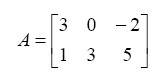
>> A = [3 0 -2 ; 1 3 5]
A =
3 0 -2
1 3 5A is a rectangular matrix of size 2x3.
- In Exercise 1 above, extract the element in the second row and second column of the matrix A.
>> A(2,2)
ans =
3 - In Exercise 1 above, generate a new matrix B of the same size by multiplying the matrix A by the number
>> B = 3*pi*A/2
B =
14.1372 0 -9.4248
4.7124 14.1372 23.5619 - In Exercise 3 above, extract the element in the first row and third column of the matrix B.
- In Exercise 3 above, extract the sub-matrix of the elements in common between the first and second rows and the second and third columns of the matrix B. What is the size of this new submatrix?
>> B(1:2,2:3)
ans =
0 -9.4248
14.1372 23.5619The above sub-matrix has size 2x2.
- In Exercise 3 above, determine the size of the matrix B using the MATLAB command size?
>> size(B)
ans =
2 3 - In Exercise 3 above, determine the largest of the number of rows and columns of the matrix B using the MATLAB command length?
>> length(B)
ans =
3 - In Exercise 3 above, determine the number of elements in the matrix B using the MATLAB command numel?
- In Exercise 3 above, determine the total sum of each column of the matrix B? Determine also the minimum value and the maximum value of each column of the matrix B?
>> sum(B)
ans =
18.8496 14.1372 14.1372
>> min(B)
ans =
4.7124 0 -9.4248
>> max(B)
ans =
14.1372 14.1372 23.5619 - Combine the three vectors [1 3 0 -4], [5 3 1 0], and [2 2 -1 1] to obtain a new matrix of size 3x4.
- Perform the operations of matrix addition and matrix subtraction on the following two matrices:
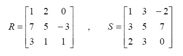
- In Exercise 11 above, multiply the two matrices R and S element-by-element.
>> R.*S
ans =
1 6 0
21 25 -21
6 3 0 - In Exercise 11 above, divide the two matrices R and S element-byelement.
>> R./S
Warning: Divide by zero.
ans =
1.0000 0.6667 0
2.3333 1.0000 -0.4286
1.5000 0.3333 InfNotice the division by zero (not allowed) above in the last element.
- In Exercise 11 above, perform the operation of matrix multiplication on the two matrices R and S. Do you get an error? Why?
>> R*S
ans =
7 13 12
16 37 21
8 17 1We do not get an error because the number of columns of the first matrix is equal to the number of rows of the second matrix.
- Add the number 5 to each element of the matrix X given below:
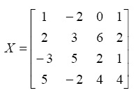
- In Exercise 15 above, subtract the number 3 from each element of the matrix X.
>> X-3
ans =
-2 -5 -3 -2
-1 0 3 -1
-6 2 -1 -2
2 -5 1 1 - In Exercise 15 above, multiply each element of the matrix X by the number -3.
>> -3*X
ans =
-3 6 0 -3
-6 -9 -18 -6
9 -15 -6 -3
-15 6 -12 -12 - In Exercise 15 above, divide each element of the matrix X by the number 2.
- In Exercise 15 above, perform the following multiple scalar operation –3* X / 2.4 + 5.5.
>> -3*X/2.4 + 5.5
ans =
4.2500 8.0000 5.5000 4.2500
3.0000 1.7500 -2.0000 3.0000
9.2500 -0.7500 3.0000 4.2500
-0.7500 8.0000 0.5000 0.5000 - Determine the sine, cosine, and tangent of the matrix B given below (element-by-element).
- In Exercise 20 above, determine the square root of the matrix B element-by-element.
>> sqrt(B)
ans =
1.0233 1.4472
1.4472 1.7725 - In Exercise 20 above, determine the true square root of the matrix B.
>> sqrtm(B)
ans =
0.5821 + 0.3598i 0.9419 - 0.2224i
0.9419 - 0.2224i 1.5240 + 0.1374iNotice that we obtained a complex matrix. Try to check this answer by multiplying this complex matrix by itself to get the original matrix.
- In Exercise 20 above, determine the exponential of the matrix B element-by-element.
- In Exercise 20 above, determine the true exponential of the matrix B.
>> expm(B)
ans =
23.9028 37.4119
37.4119 61.3147 - In Exercise 20 above, determine the natural logarithm of the matrix B element-by-element.
>> log(B)
ans =
0.0461 0.7393
0.7393 1.1447 - In Exercise 20 above, determine the true natural logarithm of the matrix B.
>> logm(B)
Warning: Principal matrix logarithm is not defined for A with
nonpositive real eigenvalues. A non-principal matrix
logarithm is returned.
> In funm at 153
In logm at 27
ans =
-0.5995 + 2.2733i 1.2912 - 1.4050i
1.2912 - 1.4050i 0.6917 + 0.8683iNotice that we obtain a non-principal complex matrix.
- In Exercise 20 above, perform the exponential operation 4B.
>> 4^B
ans =
130.0124 209.2159
209.2159 339.2283 - In Exercise 27 above, repeat the same exponential operation but this time element-by-element.
>> 4.^B
ans =
4.2705 18.2369
18.2369 77.8802 - In Exercise 20 above, perform the operation B4.
>> B^4
ans =
107.0297 173.1717
173.1717 280.2015 - Generate a rectangular matrix of 1’s of size 2x3.
- Generate a rectangular matrix of 0’s of size 2x3.
>> zeros(2,3)
ans =
0 0 0
0 0 0 - Generate a rectangular identity matrix of size 2x3.
>> eye(2,3)
ans =
1 0 0
0 1 0 - Generate a square matrix of 1’s of size 4.
>> ones(4)
ans =
1 1 1 1
1 1 1 1
1 1 1 1
1 1 1 1 - Generate a square matrix of 0’s of size 4.
- Generate a square identity matrix of size 4.
>> eye(4)
ans =
1 0 0 0
0 1 0 0
0 0 1 0
0 0 0 1 - Determine the transpose of the following matrix:
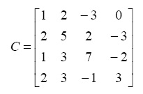
>> C = [1 2 -3 0 ; 2 5 2 -3 ; 1 3 7 -2 ; 2 3 -1 3]
C =
1 2 -3 0
2 5 2 -3
1 3 7 -2
2 3 -1 3
>> C'
ans =
1 2 1 2
2 5 3 3
-3 2 7 -1
0 -3 -2 3 -
In Exercise 36 above, perform the operation C + C'. Do you get a symmetric matrix?
>> C + C'
ans =
2 4 -2 2
4 10 5 0
-2 5 14 -3
2 0 -3 6We get a symmetric matrix.
- In Exercise 36 above, extract the diagonal of the matrix C.
>> diag(C)
ans =
1
5
7
3 - In Exercise 36 above, extract the upper triangular part and the lower triangular part of the matrix C.
- In Exercise 36 above, determine the determinant and trace of the matrix C. Do you get scalars?
>> det(C)
ans =
-13
>> trace(C)
ans =
16Both the determinant and trace are scalars (numbers in this example).
- In Exercise 36 above, determine the inverse of the matrix C.
>> inv(C)
ans =
-10.5385 6.3846 -6.0000 2.3846
5.3077 -3.0769 3.0000 -1.0769
-0.3077 0.0769 -0.0000 0.0769
1.6154 -1.1538 1.0000 -0.1538 - In Exercise 41 above, multiply the matrix C by its inverse matrix.
Do you get the identity matrix?
>> C*inv(C)
ans =
1.0000 0.0000 0.0000 0.0000
-0.0000 1.0000 0 0.0000
0 0.0000 1.0000 0
0.0000 0.0000 0 1.0000We get the identity matrix.
- In Exercise 36 above, determine the norm of the matrix C.
>> norm(C)
ans =
9.5800 - In Exercise 36 above, determine the eigenvalues of the matrix C.
>> eig(C)
ans =
-0.0702
3.9379 + 2.6615i
3.9379 - 2.6615i
8.1944We get four eigenvalues – some of them are complex numbers.
- In Exercise 36 above, determine the coefficients of the characteristic polynomial of the matrix C.
>> poly(C)
ans =
1.0000 -16.0000 86.0000 -179.0000
-13.0000We get a fourth-degree polynomial with five coefficients.
- In Exercise 36 above, determine the rank of the matrix C.
>> rank(C)
ans =
4 - Generate a square random matrix of size 5.
>> rand(5)
ans =
0.9501 0.7621 0.6154 0.4057 0.0579
0.2311 0.4565 0.7919 0.9355 0.3529
0.6068 0.0185 0.9218 0.9169 0.8132
0.4860 0.8214 0.7382 0.4103 0.0099
0.8913 0.4447 0.1763 0.8936 0.1389 - Generate a square magic matrix of size 7. What is the sum of each row, column or diagonal in this matrix.
>> magic(7)
ans =
30 39 48 1 10 19 28
38 47 7 9 18 27 29
46 6 8 17 26 35 37
5 14 16 25 34 36 45
13 15 24 33 42 44 4
21 23 32 41 43 3 12
22 31 40 49 2 11 20The sum of each row, column or diagonal is 175.
- Generate the following two symbolic matrices:
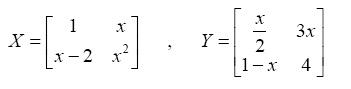
>> syms x
>> X = [1 x ; x-2 x^2]
X =
[ 1, x]
[ x-2, x^2]
>> Y = [x/2 3*x ; 1-x 4]
Y =
[ 1/2*x, 3*x]
[ 1-x, 4] - In Exercise 49 above, perform the matrix subtraction operation X – Y to obtain the new matrix Z.
>> Z = X-Y
Z =
[ 1-1/2*x, -2*x]
[ 2*x-3, x^2-4] - In Exercise 50 above, determine the transpose of the matrix Z.
In the above, it is assumed that x is a complex variable.
- In Exercise 50 above, determine the trace of the matrix Z.
>> trace(Z)
ans =
-3-1/2*x+x^2 - In Exercise 50 above, determine the determinant of the matrix Z.
>> det(Z)
ans =
5*x^2-4-1/2*x^3-4*x - In Exercise 50 above, determine the inverse of the matrix Z.
>> inv(Z)
ans =
[ -2*(x^2-4)/(-10*x^2+8+x^3+8*x),
-4*x/(-10*x^2+8+x^3+8*x)]
[ 2*(2*x-3)/(-10*x^2+8+x^3+8*x),
(x-2)/(-10*x^2+8+x^3+8*x)]The inverse of Z obtained above may be simplified by factoring out the determinant that appears common in the denominators of all the elements of the matrix.
8. Programming
- Write a script of four lines as follows: the first line should be a comment line, the second and third lines should have the assignments
cost = 200andsale_price = 250, respectively. The fourth line should have the calculationprofit = sale_price – cost. Store the script in a script file calledexample8.m. Finally run the script file.
% This is an example
cost = 200
sale_price = 250
profit = sale_price – costNow, run the above script as follows:
>> example8
cost =
200
sale_price =
250
profit =
50 - Write a function of three lines to calculate the volume of a sphere of radius
r. The first line should include the name of the function which isvolume(r). The second line should be a comment line. The third line should include the calculation of the volume of the sphere which is . Store the function in a function file called
 volume.mthen run the function with the value ofrequal to 2 (no units are used in this exercise).function volume(r)
% This is a function
volume = (4/3)*pi*r^3Now, run the above function as follows:
>> volume(2)
volume =
33.5103 - Write a function with two arguments to calculate the area of a rectangle with sides
aandb. The function should have three lines. The first line should include the name of the function which isRectangleArea(a,b). The second line should be a comment line. The third line should include the calculation of the area of the rectangle with is the producta*b. Store the function in a function file calledRectangleArea.mthen run the function twice as follow: the first execution with the values3and6, while the second execution with the values2.5and5.5.function RectangleArea(a,b)
% This is another example of a function
RectangleArea = a*bNow, run the above function as follows:
- Write a script containing a
For loopto compute the vectorxto have the values x(n) = n3 wherenhas the range from1to7. Include a comment line at the beginning. Store the script in a script file calledexample9.mthen run the script and display the values of the elements of the vectorx.% This is an example of a FOR loop
for n = 1:7
x(n) = n^3;
endNow, run the above script as follows:
>> example9
>> x
x =
1 8 27 64 125 216 343 - Write a script containing two nested
Forloops to compute the matrix y to have the values y(m,n) = m2-n2 where bothmandneach has the range from1to4. Include a comment line at the beginning. Store the script in a script file calledexample10.mthen run the script and display the values of the elements of the matrixy.%This is an example of another FOR loop
for n = 1:4
for m = 1:4
y(m,n) = m^2 - n^2;
end
endNow, run the above script as follows:
- Write a script containing a
While loopusing the two variablestolandn. Before entering theWhile loop, initialize the two variables using the assignmentstol = 0.0andn = 3. Then use the two computationsn = n + 1andtol = tol + 0.1inside theWhile loop. Make the loop end when the value oftolbecomes equal or larger than1.5. Include a comment line at the beginning. Store the script in a script file calledexample11.mthen run the script and display the values of the two variablestolandn.% This is an example of a While loop
tol = 0.0;
n = 3;
while tol < 1.5
n = n + 1;
tol = tol + 0.1;
endNow, run the above script as follows:
- Write a function called
price(items)containing anIfconstruct as follows. Let the price of the items be determined by the computationprice = items*130unless the value of the variableitemsis greater than5– then in this case the computationprice = items*160should be used instead. Include a comment line at the beginning. Store the function in a function file calledprice.mthen run the function twice with the values of3and9for the variableitems. Make sure that the function displays the results for the variableprice.function price(items)
% This is an example of an If Elseif construct
price = items*130
if items > 5
price = items*160
endNow, run the above function as follows:
>> price(3)
price =
390
>> price(9)
price =
1170
price =
1440 - Write a function called
price2(items)containing anIf Elseifconstruct as follows. If the value of the variableitemsis less than3, then compute the variableprice2by multiplyingitemsby130. In the second case, if the value of the variableitemsis less than5, then compute the variableprice2by multiplyingitemsby160. In the last case, if the value of the variableitemsis larger than5, then compute the variableprice2by multiplying theitemsby200. Include a comment line at the beginning. Store the function in a function file calledprice2.mthen run the function three times – with the values of2, 4,and6. Make sure that the function displays the results for the variableprice2.function price2(items)
% This is an example of an If Elseif construct
if items < 3
price2 = items*130
elseif items < 5
price2 = items*160
elseif items > 5
price2 = items*200
endNow, run the above function as follows:
- Write a function called
price3(items)containing aSwitch Caseconstruct. The function should produce the same results obtained in Exercise 8 above. Include a comment line at the beginning. Store the function in a function file calledprice3.mthen run the function three times – with the values of2, 4, and6. Make sure that the function displays the results for the variableprice3.function price3(items)
% This is an example of the Switch Case construct
switch items
case 2
price3 = items* 130
case 4
price3 = items* 160
case 6
price3 = items* 200
otherwise
price3 = 0
endNow, run the above function as follows:
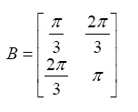
- Write a script file to store the following symbolic matrix
Athen calculate its third power B = A3. Include a comment line at the beginning. Store the script in a script file calledexample12.mthen run the script to display the two matricesAandB.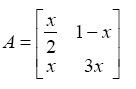
% This is an example with the Symbolic
Math Toolbox
syms x
A = [x/2 1-x ; x 3*x]
B = A^3Now, run the above script as follows:
>> example12
A =
[1/2*x, 1-x]
[ x, 3*x]
B =
[ 1/2*x*(1/4*x^2+(1-x)*x)+7/2*(1-x)*x^2,
7/4*(1-x)*x^2+(1-x)*((1-x)*x+9*x^2)]
[ x*(1/4*x^2+(1-x)*x)+21/2*x^3,
7/2*(1-x)*x^2+3*x*((1-x)*x+9*x^2)] - Write a function called
SquareRoot2(matrix)similar to the functionSquareRoot(matrix)described at the end of this chapter but with the following change. Substitute the value of1.5instead of1for the symbolic variablex. Make sure that you include a comment line at the beginning. Store the function in a function file calledSquareRoot2.mthen run the function using the following symbolic matrix: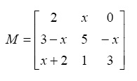
function SquareRoot2(matrix)
% This is an example of a function
with the Symbolic Math Toolbox
y = det(matrix)
z = subs(y,1.5)
if z < 1
M = 2*sqrt(matrix)
else
M = sqrt(matrix)
endNow, run the above function as follows:
9. Graphs
Solve all the exercises using MATLAB. All the needed MATLAB commands for these exercises were presented in this chapter.
- Plot a two-dimensional graph of the two vectors x = [1 2 3 4 5 6 7] and y = [10 15 23 43 30 10 12] using the plot command.
>> x = [1 2 3 4 5 6 7]
x =
1 2 3 4 5 6 7
>> y = [10 15 23 43 30 10 12]
y =
10 15 23 43 30 10 12
>> plot(x,y)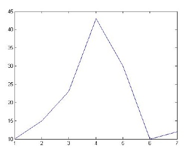
- In Exercise 1 above, add to the graph a suitable title along with labels for the x-axis and the y-axis.
>> hold on;
>> title('This is an exercise')
>> xlabel('x-axis')
>> ylabel('y-axis')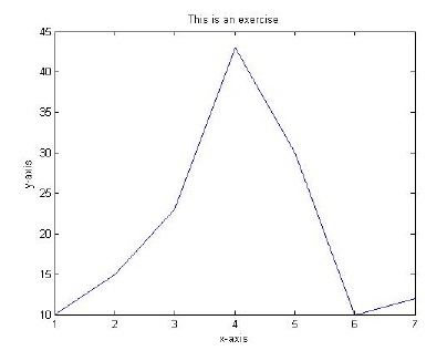
-
Plot the mathematical function y = 2x3 + 5 in the range
xfrom -6 to +6. Include a title for the graph as well as labels for the two axes.>> x = [-6 -5 -4 -3 -2 -1 0 1 2 3 4 5 6];
>> y = 2*x.^3 +5;
>> plot(x,y)
>> hold on;
>> title('This is another exercise')
>> xlabel('values of x')
>> ylabel('values of y')
- Repeat the plot of Exercise 3 above but show the curve with a blue dashed line with circle symbols at the plotted points.
plot(x,y,'b--o')
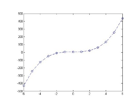
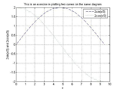
- Plot the two mathematical functions
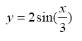 and
and 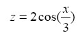 such that the two curves appear on the same 3 diagram. Make the range for
 xbetween 0 and 3π with increments of Distinguish the two curves by plotting one with a dashed line and the other one with a dotted line. Include the title and axis information on the graph as well as a grid and a legend.
>> x = 0:pi/4:3*pi;
>> y = 2*sin(x/3);
>> z = 2*cos(x/3);
>> plot(x,y,'--',x,z,':')
>> hold on;
>> grid on;
>> title('This is an exercise in plotting two curves on the same diagram')
>> xlabel('x')
>> ylabel('2sin(x/3) and 2cos(x/3)')
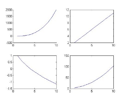
>> legend('2sin(x/3)','2cos(x/3)') - Plot the following four mathematical functions each with its own diagram using the
subplotcommand. The functions are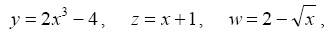 and v = x2 + 3. Use the vector x = [1 2 3 4 5 6 7 8 9 10] as the range for x. No need to show title or axis information.
>> x = [1 2 3 4 5 6 7 8 9 10];
>> y = 2*x.^3 -4;
>> z = x+1;
>> w = 2 - sqrt(x);
>> v = x.^2 +3;
>> subplot(2,2,1);
>> hold on;
>> plot(x,y);
>> subplot(2,2,2);
>> plot(x,z);
>> subplot(2,2,3);
>> plot(x,w);
>> subplot(2,2,4);
>> plot(x,v); - Use the
plot3command to show a three-dimensional curve of the equation z = 2sin(xy). Use the vector x = [1 2 3 4 5 6 7 8 9 10] for bothxandy. No need to show title or axis information.>> x = [1 2 3 4 5 6 7 8 9 10];
>> y = [1 2 3 4 5 6 7 8 9 10];
>> z = 2*sin(x.*y);
>> plot3(x,y,z)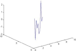
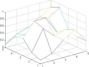
- Use the
meshcommand to plot a three-dimensional mesh surface of elements of the matrixMgiven below. No need to show title or axis information.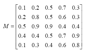
>> M = [0.1 0.2 0.5 0.7 0.3 ; 0.2 0.8 0.5 0.6 0.3 ; 0.5 0.9 0.9 0.4 0.4 ; 0.4 0.4 0.5 0.7 0.9 ; 0.1 0.3 0.4 0.6 0.8]
M =
0.1000 0.2000 0.5000 0.7000 0.3000
0.2000 0.8000 0.5000 0.6000 0.3000
0.5000 0.9000 0.9000 0.4000 0.4000
0.4000 0.4000 0.5000 0.7000 0.9000
0.1000 0.3000 0.4000 0.6000 0.8000
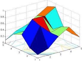
>> mesh(M) - Use the
surfcommand to plot a three-dimensional surface of the elements of the matrixMgiven in Exercise 8 above. No need to show title or axis information.>> surf(M)

- Use the
contourcommand to plot a contour map of the elements of the matrixMgiven in Exercise 8 above. No need to show the contour values on the graph.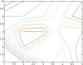
- Use the
surfccommand to plot a three-dimensional surface along with contours underneath it of the matrixMgiven in Exercise 8 above. No need to show title or axis information.>> surfc(M)
- Solve the following linear algebraic equation for the variable x. Use the roots command.
3x + 5 = 0
>> p = [3 5]
p =
3 5
>> roots(p)
ans =
-1.6667 - Solve the following quadratic algebraic equation for the variable x. Use the roots command.
x2 + x +1 = 0
>> p = [1 1 1]
p =
1 1 1
>> roots(p)
ans =
-0.5000 + 0.8660i
-0.5000 - 0.8660i - Solve the following algebraic equation for x. Use the roots command.
3x4 - 2x3 + x - 3 = 0
>> p = [3 -2 0 1 -3]
p =
3 -2 0 1 -3
>> roots(p)
ans =
1.1170
0.2426 + 0.9477i
0.2426 - 0.9477i
-0.9355 - Solve the following system of linear simultaneous algebraic equations for the variables x and y. Use the inverse matrix method.
3x + 5y = 9
4x - 7y = 13 - In Exercise 4 above, solve the same linear system again but using the Gaussian elimination method with the backslash operator.
>> A = [3 5 ; 4 -7]
A =
3 5
4 -7
>> b = [9 ; 13]
b =
9
13
>> x = A\b
x =
3.1220
-0.0732 - Solve the following system of linear simultaneous algebraic equations for the variables x, y, and z. Use Gaussian elimination with the backslash operator.
2x - y + 3z = 5
4x + 5z = 12
x + y + 2z = -3 - Solve the following linear algebraic equation for the variable x in terms of the constant a.
2x + a = 5
>> syms x
>> syms a
>> solve('2*x + a - 5 = 0')
ans =
-1/2*a+5/2 - Solve the following quadratic algebraic equation for the variable x in terms of the constants a and b.
x2 + ax + b = 0
>> syms x
>> syms a
>> syms b
>> solve('x^2 + a*x + b = 0')
ans =
-1/2*a+1/2*(a^2-4*b)^(1/2)
-1/2*a-1/2*(a^2-4*b)^(1/2) - Solve the following nonlinear equation for the variable x.
2ex+ 3cos x = 0
>> syms x
>> solve('2*exp(x) + 3*cos(x) = 0')
ans =
-1.6936679094546100269188394124169The above answer is approximated as -1.694.
- Solve the following system of linear simultaneous algebraic equations for the variables x and y in terms of the constant c.
2x − 3cy =5
cx + 2y =7 - Solve the following system of nonlinear simultaneous algebraic equations for the variables x and y.
3 x2 − 2+ + y = 7
xy + x = 5>> syms x
>> syms y
>> [x,y] = solve('3*x^2 - 2*x + y - 7 = 0', 'x*y + x - 5 = 0')
x
= 5/3
1/2*5^(1/2)-1/2
-1/2-1/2*5^(1/2)
y =
2
3/2+5/2*5^(1/2)
3/2-5/2*5^(1/2)
11. Beginning Calculus
- Define the following mathematical function in MATLAB using the
inlinecommand:
f (x) = 3x2 + x - 1
- In Exercise 1 above, evaluate the function
fat x = 1.>> f(1)
ans =
3 - In Exercise 1 above, evaluate the function
fat x = –2.>> f(-2)
ans =
9 - In Exercise 1 above, differentiate the function
fwith respect tox.>> syms x
>> diff(f(x),x)
ans =
6*x+1 - Define the following mathematical function in MATLAB using the
inline command:
g(y) = 2sin(πy) + 3y cos(πy)
- In Exercise 5 above, differentiate the function
gwith respect toy.>> diff(g(y),y)
ans =
2*cos(pi*y)*pi+3*cos(pi*y)-3*y*sin(pi*y)*pi - In Exercise 5 above, find the indefinite integral of the function
g.>> int(g(y))
ans =
-
2/pi*cos(pi*y)+3/pi^2*(cos(pi*y)+y*sin(pi*y )*pi) - In Exercise 5 above, find the value of the following definite integral

>> int(g(y),0,1)
ans =
2*(2*pi-3)/pi^2 -
In Exercise 8 above, evaluate the value obtained numerically using the
double command. - Evaluate the following limit in MATLAB:
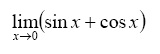
>> limit(sin(x)+cos(x),x,0)
ans =
1 - Evaluate the following limit in MATLAB:
>> limit((x^2+x+1)/(3*x^2-2),x,Inf)
ans =
1/3 - Find the Taylor series expansion for the function cos x up to eight terms.
>> taylor(cos(x),x,8)
ans =
1-1/2*x^2+1/24*x^4-1/720*x^6 - Find the Taylor series expansion for the function ex up to nine terms.
- Evaluate the following sum symbolically using the symsum command:

>> syms k
>> syms n
>> symsum(1/k,1,n)
ans =
Psi(n+1)+eulergammaThe above result is written in terms of special functions. Consult a book on special function for more details.
- Solve the following initial value ordinary differential equation using the
dsolvecommand:
>> dsolve('Dy = x*y - sin(x) + 3', 'y(0)=0')
ans =
(sin(x)-3+exp(x*t)*(-sin(x)+3))/x