4. Mathematical Functions

In this chapter we introduce the use of mathematical functions in MATLAB. These functions include the square root function, the factorial, the trigonometric functions, the exponential functions, and the rounding and remainder functions 7. We will start with the square root function⁸ used with the MATLAB command sqrt as follows:

>> sqrt(2)

ans =

1.4142

The above result gives the value of . The factorial of an integer is obtained using the MATLAB command factorial as follows:

>> factorial(5)

ans =

120

All the trigonometric functions are also available within MATLAB. For example the sine and cosine functions are used with the MATLAB commands sin and cos as follows:

>> sin(30)

ans =

-0.9880

>> sin(30*pi/180)

ans =

0.5000

>> cos(30*pi/180)

ans =

0.8660

Note that the argument for the trigonometric functions must be in radians. Check the first example above to see that the sine of the angle of 30 radians is -0.9880 but the sine of the angle of 30 degrees (converted into radians by multiplying it by ) is 0.5. The cosine of the angle of 30 degrees is seen above to be 0.8660. In addition, the tangent function is represented using the MATLAB command tan as follows where we compute the tangent of the angle of 30 degrees:

>> tan(30*pi/180)

ans =

0.5774

The other trigonometric functions of secant, cosecant and cotangent are all represented in MATLAB using the commands sec, csc, and cot. In addition, the inverse trigonometric functions are represented by the MATLAB commands asin, acos, atan, asec, acsc, and acot. For example, the inverse tangent function is calculated as follows:

>> atan(1)

ans =

0.7854

The angle returned in the above example is in radians. The hyperbolic trigonometric functions are represented by the MATLAB commands sinh, cosh, tanh, sech, csch, and coth. In addition, the inverse hyperbolic trigonometric functions are represented by the MATLAB commands asinh, acosh, atanh, asech, acsch, and acoth. Using these commands in MATLAB is straightforward. However, you need to consult a book on mathematics or trigonometry to check any limitations on the arguments of these functions. For example, if you try to find the tangent of the angle (90 degrees), then you will get a very large quantity as follows:

>> tan(pi/2)

ans =

1.6331e+016

The reason for the strange result above is that the tangent function is not defined for the angle 90 degrees and the result given by MATLAB approaches infinity (thus we get a very large quantity).

The exponential and logarithmic functions are also represented by MATLAB. For example, the exponential function is represented by the MATLAB command exp as follows:

>> exp(1)

ans =

2.7183

The above result gives the value of e¹ . There are several logarithmic functions available in MATLAB. For example, the natural logarithm is represented by the command log and the logarithm to the base 10 is represented by the command log10. Here are two examples to illustrate this:

>> log(4)

ans =

1.3863

>> log10(4)

ans =

l0.6021

The above two results give the values of ln 4 and log₁₀ 4. We may also use the MATLAB command log2 to obtain the logarithm to the base 2. For example, log2(4) will result in the value for log₂ 4 =2.

Several rounding and remainder functions are also available in MATLAB. These functions are represented by the MATLAB commands fix, floor, ceil, round, mod, rem, and sign. For example, the rounding function round and the remainder function rem are used as follows:

>> round(4.57)

ans =

5

>> rem(10,4)

ans =

2

The above result gives the remainder when dividing 10 by 4. Finally, the absolute value function is represented by the MATLAB command abs as shown in the following example:

>> abs(-7)

ans =

7

There are numerous other functions available in MATLAB like the complex functions which will be covered in the next chapter. Also, there are functions for coordinate transformations and there are number theoretic functions but these are beyond the scope of this book.

Mathematical functions can be combined using several commands on the same line in MATLAB and used with arithmetic operations. Here are some examples:

>> 2 + sqrt(5.3/3)

ans =

3.3292

>> sin(cos(3.2))

ans =

-0.8405

>> 2*log(2)/tan(pi/16)

ans =

6.9694

The important point to consider when dealing with mathematical functions is to know what type of argument is valid for each function. For example, if you try to compute the natural logarithm of zero, then you will get an error or minus infinity because this function is not defined for zero. Here is the result:

>> log(0)
Warning: Log of zero.

ans =

-Inf

Finally, mathematical functions can be used with variables. Here is an example:

>> a = 5

a =

5

>> b = 2

b =

2

>> c = b - sqrt(a+b/2)

c =

-0.4495

Mathematical Functions with the MATLAB Symbolic Math Toolbox

Mathematical functions can also be used with the MATLAB Symbolic Math Toolbox. For example, the square root of 40 can be computed symbolically without performing any numerical calculations as follows:

>> sym(sqrt(40))

ans =

sqrt(40)

>> simplify(ans)

ans =

2*10^(1/2)

In the above, the simplify command is used to obtain the square root of 40 as 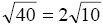. To obtain a numerical result, use the double command applied on the previous result as follows:

>> double(ans)

ans =

6.3246

The sine and cosine of the angle 30 degrees are computed symbolically as follows:

>> sym(sin(30*pi/180))

ans =

1/2

>> sym(cos(30*pi/180))

ans =

sqrt(3/4)

In addition, the tangent of the angle 30 degrees is obtained symbolically as follows:

>> sym(tan(30*pi/180))

ans =

sqrt(1/3)

Finally, the exponential and logarithm functions can also be used with Symbolic Math Toolbox. For example, the following command will compute e^2π symbolically:

>> sym(exp(2*pi))

ans =

4710234414611992*2^(-43)

In order to obtain a numerical result, use the double command applied to the previous answer as follows:

>> double(ans)

ans =

535.4917

In the next chapter, we will introduce complex numbers in MATLAB and how to handle them using complex functions

Exercises

Solve all the exercises using MATLAB. All the needed MATLAB commands for these exercises were presented in this chapter. Note that Exercises 19-25 require the use of the MATLAB Symbolic Math Toolbox.

Compute the square root of 10.

Compute the factorial of 7.

Compute the cosine of the angle 45 where 45 is in radians.

Compute the cosine of the angle 45 where 45 is in degrees.

Compute the sine of the angle of 45 where 45 is in degrees.

Compute the tangent of the angle 45 where 45 is in degrees.

Compute the inverse tangent of 1.5.