7. Matrices
In this chapter we introduce matrices and how to deal with them in MATLAB. Matrices are stored as two-dimensional arrays14 in MATLAB. A matrix is a collection of numbers and/or scalars arranged in rows and columns. For example here is a matrix of numbers with three rows and four columns:
>> x = [2 1 -3 0 ; -2 3 4 1 ; 5 -2 1 3]
x =
2 1 -3 0
-2 3 4 1
5 -2 1 3
In the above example, the matrix x is rectangular because the number of columns and the number of rows are not equal. In the specification of the matrix in MATLAB, the elements of the same row are separated by spaces while the rows themselves are separated by semicolons. Brackets are used to indicate the beginning and end of a matrix. In particular, the above matrix is called a 3x4 rectangular matrix.
We may extract the element in the second row and the third column by using the notation x(2,3) as follows:
>> x(2,3)
ans =
4
We may also extract the element in the first row and the fourth column as follows
>> x(1,4)
ans =
0
A new matrix of the same size (i.e the same number of rows and columns) may be generated by multiplying the matrix by a number as follows:
>> y = 2*pi*x
y =
We may extract the element in the third row and the third column of the matrix y as follows:
>> y(3,3)
ans =
6.2832
We may also extract the elements common in the first and second rows and the second and third columns of the matrix y as follows:
In the above example, we obtain a sub-matrix of size 2x2, i.e. with two rows and two columns. The size of a matrix is the number of rows and columns of the matrix. This is determined in MATLAB by using the command size as follows:
>> size(y)
ans =
3 4
In the above example, we obtain two numbers – the first one is the number of rows while the second one is the number of columns. The MATLAB command length may also be used but it gives one number – the largest of the number of rows and the number of columns. Here is an example:
>> length(y)
ans =
4
In the above example, we obtain the single number 4, i.e. the largest of 3 and 4. The number of elements in a matrix is obtained by using the MATLAB command numel as follows:
>> numel(y)
ans =
12
In the above example, we obtain 12 which is the product of 3 and 4 – the total number of elements in the matrix. The MATLAB commands sum, min, and max may also be used as follows:
>> sum(y)
ans =
31.4159 12.5664 12.5664 25.1327
>> min(y)
ans =
-12.5664 -12.5664 -18.8496 0
>> max(y)
ans =
31.4159 18.8496 25.1327 18.8496
In the above example, the MATLAB command sum gives the total sum of each column of the matrix, the MATLAB command min gives the minimum value of each column of the matrix, while the MATLAB command max gives the maximum value of each column of the matrix.
We can combine two or more matrices to obtain a new matrix. Here is an example of how to combine two vectors to obtain a matrix:
We can perform certain operation on matrices. For example, we can perform the operations of matrix addition and matrix subtraction on two matrices of the same size. Here is an example:
>> x = [0.2 -0.1 ; 1.3 0.0 ; 2.4 -1.5]
x =
0.2000 -0.1000
1.3000 0
2.4000 -1.5000
>> y = [0.5 1.0 ; 1.2 1.3 ; -2.0 1.3]
y =
0.5000 1.0000
1.2000 1.3000
-2.0000 1.3000
>> x+y
ans =
0.7000
0.9000
2.5000 1.3000
0.4000 -0.2000
>> x-y
ans =
-0.3000 -1.1000
0.1000 -1.3000
4.4000 -2.8000
In the above example, we added and subtracted two rectangular matrices of size 3x2. You will get an error message if you try to add or subtract two matrices of different sizes.
Matrix multiplication is not defined for two matrices of the same size (unless they are square matrices). You will get an error message if you try to multiply two matrices of the same size. Here is an example:
>> x*y
??? Error using ==> mtimes
Inner matrix dimensions must agree.
However, you can multiply two matrices of the same size element-by-element by adding the dot symbol before the multiplication symbol as follows:
>> x.*y
ans =
0.1000 -0.1000
1.5600 0
-4.8000 -1.9500
The resulting matrix above is of the same size as the two matrices that were multiplied. Division of matrices is absolutely not defined mathematically15. You will get an error message if you try to divide two matrices of any size. However, you may divide two matrices of the same size element-by-element by including the dot symbol before the division symbol as follows:
>> x./y
ans =
0.4000 -0.1000
1.0833 0
-1.2000 -1.1538
The resulting matrix above is of the same size as the two matrices that were divided. Next, we discuss the multiplication of matrices. Two matrices may be multiplied if the number of columns of the first matrix equals the number of rows of the second matrix. Here is an example:
>> u = [1 3 ; -2 0 ; 1 5]
u =
1 3
-2 0
1 5
>> v = [3 4 1 -2 ; 1 0 -1 2]
v =
3 4 1 -2
1 0 -1 2
>> u*v
ans =
6 4 -2 4
-6 -8 -2 4
8 4 -4 8
In the above example, we multiplied a 3x2 matrix by a 2x4 matrix to obtain a 3x4 matrix. It is clear that the rule of matrix multiplication applies in this case.
Next, we discuss the operations of scalar addition, scalar subtraction, scalar multiplication, and scalar division. A scalar can be added or subtracted from a matrix as follows:
>> s = [1 3 -2 5 ; 2 6 -3 0]
s =
1 3 -2 5
2 6 -3 0
>> s+5
ans =
6 8 3 10
7 11 2 5
>> s-2
ans =
-1 1 -4 3
0 4 -5 -2
In the above scalar addition and scalar subtraction operations, the number 5 was added to each element of the matrix s, while the number 2 was subtracted from each element of the matrix s. Scalar multiplication and scalar division may be performed in the same way as follows:
>> s*3
ans =
3 9 -6 15
6 18 -9 0
>> s/4
ans =
0.2500 0.7500 -0.5000 1.2500
0.5000 1.5000 -0.7500 0
In the above example, the number 3 was multiplied by each element of the matrix s, while the each element of the matrix s was divided by the number 4. In addition, multiple scalar operations may be performed on the same line as follows:
>> 3 - 2*s/1.5
ans =
1.6667 -1.0000 5.6667 -3.6667
0.3333 -5.0000 7.0000 3.0000
Mathematical functions can also be used with matrices. In the following example, we use the trigonometric functions of sine, cosine, and tangent. All the calculations are performed element-by-element using the MATLAB commands sin, cos, and tan as follows:
>> w = [0 pi/2 pi ; pi/2 pi 3*pi/2 ; pi 3*pi/2 2*pi]
w =
0 1.5708 3.1416
1.5708 3.1416 4.7124
3.1416 4.7124 6.2832
>> sin(w)
ans =
0 1.0000 0.0000
1.0000 0.0000 -1.0000
0.0000 -1.0000 -0.0000
>> cos(w)
ans =
1.0000 0.0000 -1.0000
0.0000 -1.0000 -0.0000
-1.0000 -0.0000 1.0000
>> tan(w)
ans =
1.0e+016 *
0 1.6331 -0.0000
1.6331 -0.0000 0.5444
-0.0000 0.5444 -0.0000
The square root of a matrix can also be calculated in MATLAB using two different approaches. In the first approach, the square root is calculated using the usual MATLAB command sqrt with the computations performed element-by-element as follows:
>> sqrt(w)
ans =
0 1.2533 1.7725
1.2533 1.7725 2.1708
1.7725 2.1708 2.5066
However, in the above example we do not obtain a true square root of the matrix. In order to find the true square root of the matrix, we need to use the special matrix MATLAB command sqrtm as follows:
>> sqrtm(w)
ans =
0.3086 + 0.8659i 0.5476 + 0.1952i 0.7867 - 0.4755i
0.5476 + 0.1952i 0.9718 + 0.0440i
1.3960 - 0.1072i
0.7867 - 0.4755i 1.3960 - 0.1072i 2.0053 + 0.2612i
Obviously, the result above is a complex matrix. If you try to multiply it by itself, you will obtain the original matrix. Similarly, there are two MATLAB commands for computing the exponential of a matrix. The first one is the usual command exp which performs the calculations element-by-element as follows:
>> exp(w)
ans =
1.0000 4.8105 23.1407
4.8105 23.1407 111.3178
23.1407 111.3178 535.4917
However, in order to obtain a true exponential of a matrix, the special command of expm should be used as follows:
>> expm(w)
ans =
1.0e+004 *
0.4586 0.8138 1.1690
0.8138 1.4442 2.0745
1.1690 2.0745 2.9801
Similarly, there are two MATLAB commands for computing the natural logarithm of a matrix. The first one is the usual command of log which performs the calculations element-by-element as follows:
>> log(w)
Warning: Log of zero.
ans =
-Inf 0.4516 1.1447
0.4516 1.1447 1.5502
1.1447 1.5502 1.8379
Note that the first element in the resulting matrix above is minus infinity – this is because we are trying to compute the natural logarithm of zero which is not defined. However, in order to obtain a true natural logarithm of a matrix, the special command of logm should be used as follows:
>> logm(w)
Warning: Principal matrix logarithm is not defined for A with
nonpositive real eigenvalues. A non-principal matrix
logarithm is returned.
> In funm at 153
In logm at 27
ans =
-5.9054 + 2.8465i 13.1738 - 0.5236i - 5.9209 - 0.7521i
13.1738 - 0.5236i -24.7338 + 2.2124i 13.7066 - 1.3348i
-5.9209 - 0.7521i 13.7066 - 1.3348i - 4.8399 + 1.2242i
Obviously, a complex matrix is generated as the true natural logarithm. Note the remark generated by MATLAB which says that the natural logarithm that is generated is non-principal. We can also perform the following exponential operation:
The above exponential operation may also be performed element-by-element by including the dot symbol as follows:
>> 2.^w
ans =
1.0000 2.9707 8.8250
2.9707 8.8250 26.2162
8.8250 26.2162 77.8802
Other operations may also be performed on the matrix w. For example, the cube of the matrix w, which is w3 may be obtained as follows:
>> w^3
ans =
116.2735 209.2924 302.3112
209.2924 372.0753 534.8583
302.3112 534.8583 767.4053
There are some standard matrices that can be generated automatically by MATLAB. For example, matrices with elements of 1’s and 0’s can be generated using the commands ones and zeros as follows:
In addition, a special matrix called the identity matrix16 can be generated using the MATLAB command eye as follows:
>> eye(3,5)
ans =
1 0 0 0 0
0 1 0 0 0
0 0 1 0 0
A matrix with the same number of rows and columns is called a square matrix. For example, a matrix with three rows and three columns is called a square matrix of size 3. Here is an example:
>> m = [1 4 -2 ; 0 4 7 ; 1 -2 5]
m =
1 4 -2
0 4 7
1 -2 5
For the remaining part of this discussion, we will deal with operations and handling of square matrices. For example, the above three commands of ones, zeros, and eye can be used as follows to generated standard square matrices as follows:
>> ones(3)
ans =
1 1 1
1 1 1
1 1 1
>> zeros(3)
ans =
0 0 0
0 0 0
0 0 0
>> eye(3)
ans =
1 0 0
0 1 0
0 0 1
Notice the different usage of the above three commands when used to generate square matrices. The operations and commands that we will discuss next are part of the subject called matrix algebra. We will not provide a comprehensive coverage of this subject here, but we will provide the essential commands. The transpose of a matrix is generated in MATLAB using the prime symbol as follows:
In the above example, A’ is the transpose17 of A. It is generated by replacing each row in A with its corresponding column. In effect, the rows and columns are switched. For example, we next add the matrix A with its transpose:
>> A+A'
ans =
2 1 7
1 10 2
7 2 12
Note that the resulting matrix is symmetric. The diagonal of a square matrix can be extracted using the MATLAB command diag as follows:
We can also extract the upper triangular part and the lower triangular part18 of the matrix using the MATLAB commands triu and tril as follows:
>> triu(A)
ans =
1 3 6
0 5 0
0 0 6
>> tril(A)
ans =
1 0 0
-2 5 0
1 2 6
The determinant and inverse of a matrix are obtained by using the MATLAB commands det and inv as follows:
Note that the determinant is always a scalar (a number in this case) while the inverse of a square matrix is also a square matrix of the same size. If we multiply the matrix by its inverse matrix, we should obtain the identity matrix of the same size as follows:
>> A*inv(A)
ans =
1.0000 -0.0000 0
-0.0000 1.0000 0.0000
-0.0000 -0.0000 1.0000
We can obtain the trace of a matrix using the MATLAB command trace as follows:
>> trace(A)
ans =
12
The trace19 of a matrix is the sum of the diagonal elements. It is always a scalar (a number in this case). The norm20 of a matrix can also be computed using the MATLAB command norm as follows:
Note from the example above that the norm of a matrix is always a scalar (a number in this case). We can also obtain the eigenvalues21 of the matrix A using the MATLAB command eig as follows:
>> eig(A)
ans =
0.3223
5.8389 + 1.7732i
5.8389 - 1.7732i
Note from the example above that we obtained three eigenvalues because the size of the matrix A is 3. Note also that some of the eigenvalues are complex numbers. We can also obtain the characteristic polynomial22 of the matrix A using the MATLAB command poly as follows:
>> poly(A)
ans =
1.0000 -12.0000 41.0000 -12.0000
Notice in the above result that we obtained the coefficients of the characteristic polynomial of the matrix A. Because A is a square matrix of size 3, its characteristic polynomial is cubic. Thus we obtain four coefficients for a cubic polynomial. We can obtain the rank of a matrix using the MATLAB command rank as follows:
>> rank(A)
ans =
3
For a square matrix, the rank is the same as the size of the matrix. Finally, we will discuss briefly random matrices and magic matrices. To generate a random matrix (a matrix with random elements), we use the MATLAB command rand as follows:
>> rand(3)
ans =
0.9501 0.4860 0.4565
0.2311 0.8913 0.0185
0.6068 0.7621 0.8214
As seen from the above example, the random elements of the matrix have values between 0 and 1. Of course, these values can be manipulated using the different matrix operations discussed previously in this chapter. And to generate a magic matrix (called a magic square), we use the MATLAB command magic as follows:
The above magic square of size 3x3 has the feature that the sum of any column or row or diagonal is always the same number – in this example the sum is 15.
Matrices with the MATLAB Symbolic Math Toolbox
In this section we introduce symbolic matrices, i.e. matrices with symbolic variables that can be handled algebraically without performing any numerical computations. Most of the operations and commands discussed previously in this chapter can be used with symbolic matrices. Here is an example of a symbolic square matrix of size 3 defined using the MATLAB command syms:
>> syms x
>> A = [x x-3 x^2 ; 2*x 1-x x ; 3*x 2*x-5 x^2]
A =
[ x, x-3, x^2]
[ 2*x, 1-x, x]
[ 3*x, 2*x-5, x^2]
Here is another symbolic matrix based on the same symbolic variable x:
Next, we sum the two symbolic matrices A and B to obtain the new symbolic matrix C as follows:
>> C = A+B
C =
[ x+1, x-3, x^2+x]
[ 2*x-2, 6-x, 1]
[ 3*x+2, 2*x-2, x^2+4]
The transpose of the symbolic matrix C is obtained using the prime symbol as follows:
>> C'
ans =
[ 1+conj(x), -2+2*conj(x), 2+3*conj(x)]
[ -3+conj(x), 6-conj(x), -2+2*conj(x)]
[ conj(x^2+x), 1, 4+conj(x)^2]
The determinant of the symbolic matrix C is obtained using the MATLAB command det as follows:
>> det(C)
ans =
-4*x^3+37*x+4*x^4-4-43*x^2
The trace of the symbolic matrix C is obtained using the MATLAB command trace as follows:
Finally, the inverse of the symbolic matrix C can be obtained using the MATLAB command inv as follows:
>> inv(C)
ans =
[ -(-6*x^2-26+x^3+6*x)/(-4*x^3+37*x+4*x^4-4-43*x^2), (x^3+3*x^2-6*x+12)/(-4*x^3+37*x+4*x^4-4-43*x^2), (-5*x-3-5*x^2+x^3)/(-4*x^3+37*x+4*x^4-4-43*x^2)]
[ -(2*x^3-2*x^2+5*x-10)/(-4*x^3+37*x+4*x^4-4-43*x^2), -2*(x^3+2*x^2-x-2)/(-4*x^3+37*x+4*x^4-4-43*x^2), (2*x^3-3*x-1)/(-4*x^3+37*x+4*x^4-4-43*x^2)]
[ (7*x^2-24*x-8)/(-4*x^3+37*x+4*x^4-4-43*x^2), (x^2-7*x-4)/(-4*x^3+37*x+4*x^4-4-43*x^2), -x*(3*x-13)/(-4*x^3+37*x+4*x^4-4-43*x^2)]
The above expression for the inverse matrix in symbolic form is very complicated. There are techniques in MATLAB and the Symbolic Math Toolbox that can be used to simplify the above expression but will not be used here. The reason is that the above expression can be simplified by hand by factoring out the determinant that appears in the denominators of the elements of the matrix.
In the next chapter, we will discuss programming in MATLAB concentrating on using scripts and functions.
Solve all the exercises using MATLAB. All the needed MATLAB commands for these exercises were presented in this chapter. Note that Exercises 49-54 require the use of the MATLAB Symbolic Math Toolbox.
- Generate the following rectangular matrix in MATLAB. What is the size of this matrix?
- In Exercise 1 above, extract the element in the second row and second column of the matrix
A. - In Exercise 1 above, generate a new matrix B of the same size by multiplying the matrix
Aby the number .
. - In Exercise 3 above, extract the element in the first row and third column of the matrix
B. - In Exercise 3 above, extract the sub-matrix of the elements in common between the first and second rows and the second and third columns of the matrix
B. What is the size of this new sub-matrix? - In Exercise 3 above, determine the size of the matrix
Busing the MATLAB commandsize? - In Exercise 3 above, determine the largest of the number of rows and columns of the matrix
Busing the MATLAB commandlength? - In Exercise 3 above, determine the number of elements in the matrix
Busing the MATLAB commandnumel? - In Exercise 3 above, determine the total sum of each column of the matrix
B? Determine also the minimum value and the maximum value of each column of the matrixB? - Combine the three vectors [1 3 0 -4] , [5 3 1 0], and [2 2 -1 1] to obtain a new matrix of size 3x4.
- Perform the operations of matrix addition and matrix subtraction on the following two matrices:
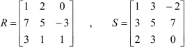
- In Exercise 11 above, multiply the two matrices
RandSelement-by-element. - In Exercise 11 above, divide the two matrices
RandSelement-by-element. - In Exercise 11 above, perform the operation of matrix multiplication on the two matrices
RandS. Do you get an error? Why? - Add the number
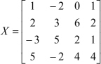
5to each element of the matrixXgiven below: - In Exercise 15 above, subtract the number
3from each element of the matrixX. - In Exercise 15 above, multiply each element of the matrix
Xby the number-3. - In Exercise 15 above, divide each element of the matrix
Xby the number2. - In Exercise 15 above, perform the following multiple scalar operation − 3* X / 2.4 + 5.5 .
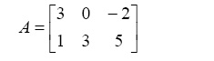
- Determine the sine, cosine, and tangent of the matrix
Bgiven below (element-by-element).
- In Exercise 20 above, determine the square root of the matrix
Belement-by-element. - In Exercise 20 above, determine the true square root of the matrix
B. - In Exercise 20 above, determine the exponential of the matrix
Belement-by-element. - In Exercise 20 above, determine the true exponential of the matrix
B. - In Exercise 20 above, determine the natural logarithm of the matrix
Belement-by-element. - In Exercise 20 above, determine the true natural logarithm of the matrix
B. - In Exercise 20 above, perform the exponential operation 4B .
- In Exercise 27 above, repeat the same exponential operation but this time element-by-element.
- In Exercise 20 above, perform the operation B4 .
- Generate a rectangular matrix of 1’s of size 2x3.
- Generate a rectangular matrix of 0’s of size 2x3.
- Generate a rectangular identity matrix of size 2x3.
- Generate a square matrix of 1’s of size 4.
- Generate a square matrix of 0’s of size 4.
- Generate a square identity matrix of size 4.
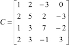
- Determine the transpose of the following matrix:
- In Exercise 36 above, perform the operation C + C' . Do you get a symmetric matrix?
- In Exercise 36 above, extract the diagonal of the matrix
C. - In Exercise 36 above, extract the upper triangular part and the lower triangular part of the matrix
C. - In Exercise 36 above, determine the determinant and trace of the matrix
C. Do you get scalars? - In Exercise 36 above, determine the inverse of the matrix
C. - In Exercise 41 above, multiply the matrix
Cby its inverse matrix. Do you get the identity matrix? - In Exercise 36 above, determine the norm of the matrix
C. - In Exercise 36 above, determine the eigenvalues of the matrix
C. - In Exercise 36 above, determine the coefficients of the characteristic polynomial of the matrix
C. - In Exercise 36 above, determine the rank of the matrix
C. - Generate a square random matrix of size 5.
- Generate a square magic matrix of size 7. What is the sum of each row, column or diagonal in this matrix.
-
Generate the following two symbolic matrices:
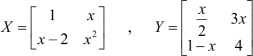
- In Exercise 49 above, perform the matrix subtraction operation X − Y to obtain the new matrix
Z. - In Exercise 50 above, determine the transpose of the matrix
Z. - In Exercise 50 above, determine the trace of the matrix
Z. - In Exercise 50 above, determine the determinant of the matrix
Z. - In Exercise 50 above, determine the inverse of the matrix
Z.