Batch Solution of Small PDEs with the OPS DSL

Abstract

In this paper we discuss the challenges and optimisations opportunities when solving a large number of small, equally sized discretised PDEs on regular grids. We present an extension of the OPS (Oxford Parallel library for Structured meshes) embedded Domain Specific Language, and show how support can be added for solving multiple systems, and how OPS makes it easy to deploy a variety of transformations and optimisations. The new capabilities in OPS allow to automatically apply data structure transformations, as well as execution schedule transformations to deliver high performance on a variety of hardware platforms. We evaluate our work on an industrially representative finance simulation on Intel CPUs, as well as NVIDIA GPUs.

1 Introduction

Traditional imperative programming languages, such as C/C++ and Fortran, still dominate computational sciences. However, these were designed for a single thread of execution in mind together with a flat memory model. In contrast, modern hardware provides massive amounts of parallelism, billions of threads in large-scale machines, at multiple levels (such as multiple cores, each with wide vectors), and a multi-level memory hierarchy or even several discrete memory spaces on a single system. Such hardware complexity need to be carefully considered for their efficient utilisation.

To allow access to new hardware features, new programming models and extensions are being introduced - the list is far too long, but the prominent models and extensions include MPI [6], OpenMP [4], CUDA [17] and OpenCL [21]. Newer models also come to light with new hardware such as the introduction of OpenACC for NVIDIA GPUs and the most recent announcement of the OneAPI model from Intel for their upcoming Xe GPUs. Such diversity in both hardware, as well as programming approaches, presents a huge challenge to computational scientists; how to productively develop code that will then be portable across different platforms and perform well on all of them. The problem appears to have no solution in the general sense, and research instead focuses on narrowing the scope, and targeting smaller problem domains. A practical concept here is the idea of separation of concerns; separate the description of what to compute from how to actually do it. The challenge then is to design a programming interface that is wide enough to support a large set of applications, but it is also narrow enough that a considerable number of assumptions can be made, and parallel execution, as well as data movement, can be organised in a variety of ways targeting different hardware.

The separation of concerns approach yields a layer of abstraction that also separates computational scientists, who use these tools, from the parallel computing experts who develop these tools, whose goal is to apply transformations and optimisations to codes using this abstraction - which given all the assumptions can be much more powerful than in the general case (i.e. what general purpose compilers can do). Domain Specific Languages in high performance computing narrow their focus on a set of well defined algorithmic patterns and data structures - OPS is one such DSL, embedded in the C/C++ and the Fortran languages. OPS presents an abstraction for describing computations on regular meshes - and application written once with the OPS API can then be automatically translated to utilise various parallel hardware using MPI, OpenMP, CUDA, OpenCL, and OpenACC.

There is a rich literature of software libraries and DSLs targeting high performance computing with the goal of performance portability. Some of the most prominent ones include KOKKOS [3] and RAJA [7], which are C++ template libraries that allow execution of loops expressed using their STL-like API on CPUs and GPUs. They also support the common Array-of-Structures to Structure-of-Arrays data layout transformation. Their approach however is limited by having to apply optimisations and transformations at compile-time, and the inability to perform cross-loop analysis (though support for task graphs has been introduced, but that is not directly applicable to the problem we study here). The ExaStencils project has also developed the ExaSlang DSL which is capable of data layout transformations and some limited execution schedule transformations [12], however their approach also does not consider batching, or the kind of cross-loop analysis and transformations that our work does.

OPS was designed to tackle a moderate number of large structured meshes, where there is sufficient parallelism within each mesh. However, there is a class of applications where computations need to be carried out on a large number of small structured meshes. This algorithmic pattern is prevalent in computational finance, where predictions need to be made given a large set of different initial conditions or other parameters. Similarly, a large fraction of computations in Adaptive Mesh Refinement (AMR) computations execute the same computations on a collection of small structured blocks. With these application domains in mind, in this paper we present an extension of the OPS abstraction that makes it practically trivial to extend an OPS application computing on a single PDE system to compute on multiple systems of the same size. We are also introducing a number of optimisations and transformations specific to situations where multiple systems are present, and expose these to the user so the most performant combination can be found easily - without requiring changes in the code. Specifically we make the following contributions:

Extend the OPS abstraction to accommodate multiple systems.
Introduce a number of data layout and execution schedule transformations applicable to the solution of multiple systems.
We develop an industrially representative financial application, and evaluate our work on Intel CPUs and NVIDIA GPUs.

The rest of the paper is organised as follows: Sect. 2 describes the OPS framework, Sect. 3 describes the extension of the OPS abstraction and the transformations and optimisations developed for batching. Section 4 describes the test application and the results, and finally Sect. 5 draws conclusions.

2 The OPS DSL

The Oxford Parallel library for Structured meshes (OPS), is a DSL embedded into C/C++ and Fortran [19]. It presents an abstraction to its users that lets them describe what to compute on a number of structured blocks, without specifying how – the details of data movement and the orchestration of parallelism are left entirely to the library, thereby achieving separation of concerns.

The abstraction allows the user to define blocks (ops_block) and describe their dimensionality (2D/3D, etc.), which serves to group datasets (ops_dat) together - these have specific extents, user-defined boundary regions, and an underlying datatype. Extents are defined by datasets rather than the blocks to allow for staggered grids and multigrid. When multiple blocks are defined, their datasets can be connected by user-defined halos (ops_halo). The user then defines a number of access patterns, or stencils (ops_stencil), that describe the pattern of access to neighbouring elements during computations later on. This information is sufficient to initialise and distribute data across different memory spaces and over MPI. The computations are then described as a parallel iteration on a given N dimensional range, executing a user-defined kernel (defined as a C or Fortran function pointer) at each point, accessing datasets using pre-defined stencils, also specifying the method of access (read/write). The parallel loop construct is ops_par_loop, with datasets passed wrapped in ops_arg_dat arguments. Mesh invariant values can be passed using the ops_arg_gbl argument to the parallel loops, and reductions with the ops_arg_reduce argument, passing in a reduction handle (ops_reduction), which can be queried separately. For a full description of the API, please refer to the user documentation [1].

../images/491247_1_En_12_Chapter/491247_1_En_12_Fig1_HTML.png — Fig. 1.
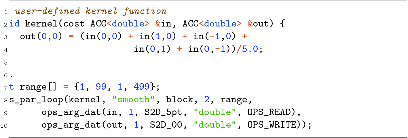
An example for an OPS parallel loop

A specific example for a parallel loop is shown in Fig. 1 - the user-defined kernel is always written from the perspective of a single iteration on the mesh, with data passed in through the templated ACC wrappers, which allow access through the overloaded parentheses operator. The only requirement regarding the user-defined kernel is that the order in which OPS iterates through the mesh must not change the end result within machine precision. This description avoids the specification of parallelism and how data gets to the user-defined kernel - the goal of OPS is to facilitate efficient parallelisation and data movement on a variety of hardware architectures, with different parallel programming models.

../images/491247_1_En_12_Chapter/491247_1_En_12_Fig2_HTML.png — Fig. 2.
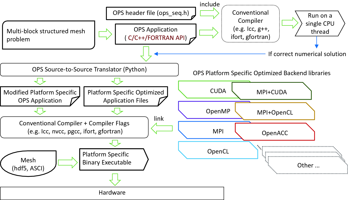
The workflow for developing an application with OPS

An OPS application written once with its high-level API can immediately be compiled with a traditional compiler and tested for correctness using a header file sequential implementation of ops_par_loop. OPS uses an “active-library” approach to parallelising on different targets; while its API looks like that of a traditional software library, it uses a combination of code generation and back-end libraries. The full OPS build system is shown in Fig. 2. The code generation step takes the user’s code, looking for calls to ops_par_loop, and parses them, gathering all information into internal data structures, that are then passed to a set of code generators targeting parallel programming methods such as OpenMP, CUDA, OpenCL, OpenACC, etc., which essentially generate the boilerplate code around the user-defined kernel, managing parallelism and data movement. These can then be compiled with target-specific compilers, and linked to the backend libraries of OPS that manage distributed and/or multiple memory spaces, and execution schedules.

During the initialisation and set-up phase of an application all mesh data is handed to OPS, and can later only be accessed through API calls. Temporaries and working arrays can be automatically allocated by OPS. While obviously limiting, it allows OPS to take full control of data management and movement. This has a number of advantages; the most prominent is the automatic distribution of data over MPI, and the management of halo exchanges - OPS is capable of running on distributed memory machines without any changes to user code, and can scale up to hundreds of thousands of cores and thousands of GPUs [11, 15]. Multiple memory spaces can also be handled automatically - such as up/downloading data to/from GPUs. The layout of data itself can also be changed with the cooperation of backend logic and code generation - a simple example is the Array-of-Structures to Structure-of-Arrays conversion, which involves the transposition itself (and changed access patterns for MPI communications) in the backend, and a different indexing scheme in the ACC data wrappers handed to the user-defined kernels.

OPS having full control over the data has another key advantage; the ability to re-schedule to order of computations - not just within a single parallel loop, but across multiple ones. The execution of an OPS application can be though of as a series of transactions that access data in clearly defined ways, and unless the control flow of the user code between calls to the OPS API is affected by data coming out of OPS, it can be perfectly reproduced. This leads to the lazy execution mechanism in OPS; calls to the OPS API are recorded and stored in a queue (without actually executing them), up to a point where data has to be returned to the user. This then triggers the execution of computations in the queue, giving OPS the ability to make transformations on an intra- and inter-loop level. We have previously used this mechanism to implement cache-blocking tiling on CPUs [18], and out-of-core computations on GPUs [20].

3 Batching Support in OPS

The key need tackled in this work is that of batching; the same computations have to be done on not just one structured block, but a large number of them. The computations are identical except for the data that is being computed on. This of course presents trivial parallelisation opportunities, and allowing for such computations in most computations is easily done. The challenge lies in achieving high performance on a variety of hardware, which may require significant data layout and execution schedule transformations - and being able to do all this without needing changes to the high level user code.

The most trivial ways to implement solving multiple systems is to either surround the entire computational code with an iteration across different systems, or just smaller code regions (such as each computational loop). This is a natural way of coding, because it allows describing computations on a single system, and the surrounding code just passes in data for different systems. This is the approach used in most existing software - perhaps most commonly in Adaptive Mesh Refinement (AMR) codes [14, 26]. The approach of surrounding several computational steps with a loop over systems is also naturally cache-friendly on CPUs, but can pose under-utilisation problems, particularly on GPUs. Loop structures with some of the common options are shown in Fig. 3.

../images/491247_1_En_12_Chapter/491247_1_En_12_Fig3_HTML.png — Fig. 3.
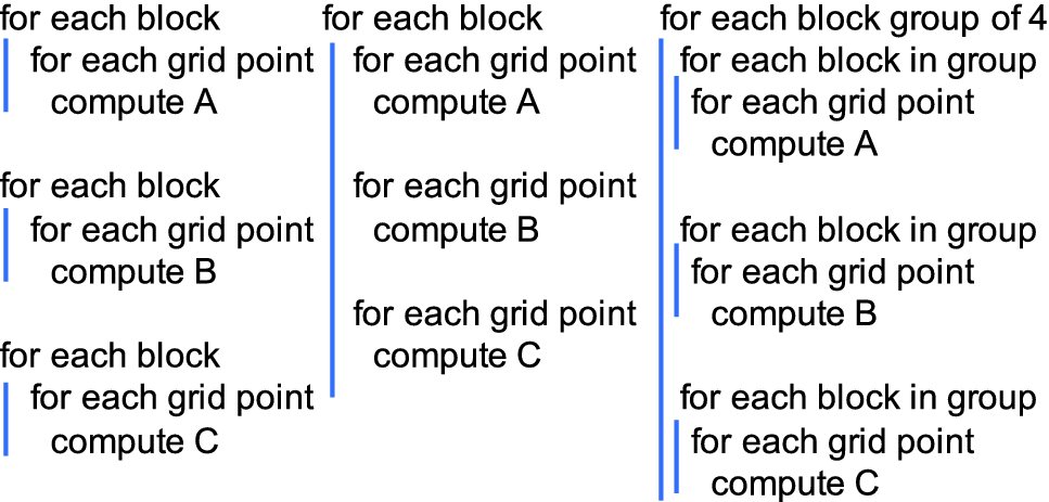
Examples of loop structure formulations when solving multiple systems

More specifically with small individual systems, there may be considerable overheads in carrying out a computational step - such as getting full vectorisation, good utilisation of prefetch engines on CPUs, or kernel launches on GPUs. This is something OPS also suffers from - the generated boilerplate code that executes and feeds the user-defined kernel has non-negligible costs, which can become significant when executing on very small blocks (100–1000 grid points). Task scheduling systems [2, 16] are also affected by this.

Another trivial approach is to extend the problem to a higher dimension, packing systems next to one another - e.g. packing multiple 2D systems into a 3D grid. While this does reduce the aforementioned overheads, it is less cache-friendly on CPUs, and may require significant code refactoring.

The challenge of appropriately arranging data for efficient execution, and scheduling computations to minimise overheads and improve data locality is highly non-trivial on any given platform, and is further complicated by the need for performance portability across multiple platforms. No implementation should therefore tie itself to a particular data structure or execution structure - this is what drove us to extend the OPS abstraction to support batching.

3.1 Extending the Abstraction

Our goals in designing extension of the abstraction were twofold: (1) a minimally intrusive change that makes it easy to extend existing applications, and (2) to allow for OPS to apply a wide range of optimisations and transformations to data layout and execution schedule.

First, we extend ops_block with an additional count field, which indicates the total number of systems. All datasets defined on these blocks will be extended to store data for each system. Furthermore, reductions need to return values of each system separately, therefore reduction handles, ops_reduction, were extended with a count field as well. The way computations in OPS are expressed is unchanged - loops are written as if they only operated on a single system. This extension allows for describing problems that are trivially batched.

However, there are situations, particularly when using iterative solvers, when certain systems no longer need to be computed upon, but others do. This necessitates the introduction of APIs that enable or disable the execution of certain systems. OPS adds two APIs - ops_par_loop_blocks_all() to indicate that computations following this point need to be carried out on all systems (which is also the default behaviour), and ops_par_loop_blocks_predicate(block, flags), which takes an array of flags to indicate which systems to execute and which ones to skip in following calls to ops_par_loop.

Semantically, the newly introduced support for multiple systems in OPS means that each ops_par_loop will be executed for each system, and each reduction will compute results for each system separately, returning an array of results (through ops_reduction_result, indexed in the same order as the systems are. From the perspective of the user, execution is done in a “bulk synchronous” way - whenever an API call is used to get data out of OPS (such as the result of a reduction), data for all the systems is returned.

In summary, an existing single-block application can be extended to work on multiple systems with the following steps:

Specify the number of systems when declaring an ops_block,
Receive multiple reduction results from OPS, one for each system,
Optionally, add the loop over blocks API calls, particularly when over time some systems are to be omitted from the calculations.

3.2 Execution Schedule Transformation

The two most trivial ways to execute multiple systems, as discussed above, is (1) for each ops_par_loop to introduce an extra loop over the different systems, and (2) to execute all ops_par_loop operations to the first system in one go, then to the second system, etc. On the level of loopnests, this maps down to having an extra loop over systems just above each spatial loop nest, or to have this loop over systems surround the whole computational code.

The first approach is trivial to implement in OPS as well, and it is indeed what the sequential header-file implementation does. It is also the preferred option for running on GPUs - launching a large grid of blocks and threads mitigates kernel launch costs. It is however not optimal on CPUs because while individual systems may fit in cache, all of them likely do not, leading to poor cache locality between subsequent ops_par_loop operations. Parallelisation on the CPU using OpenMP happens across the different systems, for each ops_par_loop separately, which also leads to unnecessary synchronisation points.

The second approach relies on the lazy execution scheme in OPS - as the code executes, loops are queued instead of being executed, and once execution is triggered, OPS iterates through all the systems, and within this iteration, all the parallel loops in the queue, passing each one the current system. CPU parallelisation is then done across different systems using OpenMP, which improves data locality between subsequent parallel loops and also removes thread synchronisation overheads. This optimisation can be enabled by defining the OPS_LAZY preprocessor macro.

When the memory footprint of a single system is small, and/or when efficient execution requires it (overheads of executing a single loop on a single system, as discussed above, e.g. efficient vectorisation on CPUs), one can create smaller batches of systems, and execute them together, thereby mitigating overheads, and making better use of caches. This is also facilitated by the lazy execution mechanism in OPS, in a similar way to the second approach described above, by passing batches of systems to each parallel loop in the queue. This number can be passed as a runtime argument to the application (OPS_BATCH_SIZE), and optionally the same preprocessor macro can be defined to make this size a compile-time constant, which enables further optimisations by the compiler.

3.3 Data Layout Transformation

The performance of computations can be significantly affected by how data is laid out and how it is accessed, and whether it aligns with the execution schedule. Considering that OPS owns all the data, it is free to make transformations to layout, and work with the generated code and the data accessor objects of OPS ( ../images/491247_1_En_12_Chapter/491247_1_En_12_Figa_HTML.gif ), so from the perspective of the user-defined kernel, these transformations are completely transparent. Given the wide array of options and target architectures, we have chosen to make these transformation options hyper-parameters - specifiable at compile- and/or run-time.

OPS expects data that is read in by the user to be passed to it when datasets are declared. Such data is supposed to follow a column major layout, and be contiguous in memory; for example for a 2D application $x\_size \times y\_size \times \#systems$ . OPS can then arbitrarily swap the axes, or even break them into multiple parts.

We first introduce the batching dimension parameter - i.e. which dimension of the $$N+1$$ dimensional tensor (N for spatial dimensions of an individual system, $$+1$$ the different systems) storing data should be used for the different systems. We have implemented code in OPS that can perform an arbitrary change of axes on input data. There are two obviously useful choices; the last dimension - the way data is given to OPS in the first place - or the first dimension, so values at the same grid point from different systems are adjacent to each other: $\#systems \times x\_size \times y\_size ...$ . The batching dimension can be set by defining the OPS_BATCHED preprocessor macro to the desired dimension index.

Keeping the batching dimension as the last dimension will keep data from the same system contiguous in memory, which lead to good data locality, but may lead to unaligned memory accesses when accessing adjacent grid points. It also means that the lowest level of parallelisation - vectorisation on CPUs, and adjacent threads on GPUs - will be on the first spatial dimension. For small systems, this may lead to underutilisation, and cause issues for auto-vectorisation.

Setting the batching dimension to be the first one makes auto-vectorisation in particular easier, as the loop over the batching dimension becomes trivially parallelisable, all accesses become aligned, and with large system counts, the utilisaiton of vector units will be high as well. It does however mean slightly more indexing arithmetic; for example in 2D, accessing a neighbour with a (i, j) offset yields the $i*\#systems + j*x\_size*\#systems$ computation. This change in indexing scheme is done in the implementation of the ACC data wrapper, and is applied at compile time. This layout also leads to jumps in memory addresses when accessing neighbouring grid points, and accessing non-contiguous memory when executing only a subset of all systems (batched execution schedule).

Finally, in situations where data locality is to be exploited, which prefers a layout with batching dimension being the last one, and vectorisation efficiency also to be improved, which prefers the layout with the batching dimension being the first one, we can use a hybrid of the two. OPS can break up the dimension of different systems into two - by forming smaller batches of systems (e.g. 4 or 8). This yields the following layout for 2D: $batch\_size \times x\_size \times y\_size \times \#systems/batch\_size$ , which can be trivially extended to higher dimensions. The batch size can be set to a multiple of the vector length on CPUs, ensuring perfect utilisation of vector units, and sized so the memory footprint fits a certain level of cache. OPS allows this parameter to be set at compile time, using the OPS_HYBRID_LAYOUT macro, allowing for better compiler optimisations - e.g. if $batch\_size$ is a power of two, integer multiplications can be replaced with bit shifts, and also no loop peeling is required for generating vectorised code.

3.4 Alternating Direction Implicit Solver

The base OPS abstraction requires that all computations are order-independent - that is, the manner in which OPS iterates through the mesh and calls the user-defined kernel, does not affect the end result. This is a reasonable requirement for most explicit methods, however many implicit methods are not implementable because of this. The alternating direction implicit (ADI) method (see e.g. [9] and the references therein) is very popular in structured mesh computations - it involves an implicit solve in alternating dimensions. We have introduced support for tridiagonal solvers (banded matrices with non-zeros on, above and below the diagonal), for which the need arises naturally from stencil computations. Tridiagonal solves are then applied in different spatial dimensions. We integrate a library which supports CPUs and GPUs [13], and write simple wrappers in OPS to its API calls; the user has to define the datasets that store the coefficients below, on, and above the diagonal, plus the right hand side, and specify the solve direction. Then, there is trivial parallelism in every other dimension, and the integrated library is additionally capable of parallelising the solution of individual systems as well using the parallel cyclic reduction (PCR) algorithm [24].

The tridiagonal solver library has a number of different implementations for solving systems that are laid out in the contiguous direction (X) - when solving many of these systems in parallel, the challenge is that their coefficients do not lend themselves to “coalesced” memory reads - which is a problem on GPUs in particular. The library offers five options for GPUs;

0.
Transpose the data using CUBLAS, and perform a Y-direction solve, then transpose the solution back,
1.
Each thread works on a different system and carries out non-coalesced reads,
2.
Load data in a coalesced way into shared memory, and transpose it there
3.
Load data in a coalesced way and use warp shuffle operations to transpose it,
4.
Load data in a coalesced way and use warp shuffle operations to transpose it, and use a hybrid Thomas-PCR algorithm to expose parallelism within a single system.

Fitting this solver in our batched extension is a matter of adding an extra dimension to the data, and solving in the appropriate dimension. When data layout is changed, the solve dimension is changed accordingly - e.g. when the batching dimension is 0, X solves become Y solves. A call to this library is represented just like any other ops_par_loop, and can be inserted into the queue during lazy execution. The wrapper takes care of selecting the correct solve dimension when the data layout is re-arranged, and passing the correct extents so the desired systems are solved.

4 Evaluation

In this section, we evaluate our work on an industrially representative computational finance application. While it does not exercise all the newly introduced features, it does help demonstrate the productivity achieved through OPS of extending support to multiple systems, and exploring the optimisation space.

4.1 The Application

In contemporary financial mathematics, stochastic local volatility (SLV) models (see e.g. [22]) constitute state-of-the-art models to describe asset price processes, notably foreign exchange rates. The model is specified via a stochastic differential equation

$\begin{aligned}&dX_t = ( r_d - r_f - 1/2 L^2(X_t,t)V_t )dt + L(X_t,t)\sqrt{V_t} dW^1_t \\&dV_t = \kappa (\eta - V_t)dt + \xi \sqrt{V_t} dW^2_t \nonumber \\&dW^1_t dW^2_t = \rho dt \nonumber \end{aligned}$

(1)

for constants $r_d, r_f, \kappa , \eta , \xi$ and $\rho$ and positive function L. $$W^1$$

and

are two independent standard Brownian motions. Note that X above is in log-space, so can be positive or negative. The process V however cannot be negative.

Using standard results from stochastic analysis, it follows that the price V of any financial contract written on X with payoff f at time 0 is given by the PDE

$\begin{aligned}{}[h]0&= V_t + \tfrac{1}{2} L^2(x,t) v V_{xx} + (r_d - r_f -\tfrac{1}{2}L^2(x,t) v) V_x \\&+ \tfrac{1}{2}\xi ^2 v V_{vv} + \kappa (\eta - v) V_v + L(x,t)\xi v\rho V_{xv} \nonumber \end{aligned}$

(2)

subject to the initial condition $$V(0,x,v) = f(x)$$

for all x and all $v\ge 0$ . Usually Dirichlet or so-called “zero gamma” boundary conditions are imposed as well. The PDE (2) is usually solved with finite differences and time integration is via an ADI time stepper, for example Modified Craig-Sneyd or Hundsdorfer-Verwer (see e.g. [10] and [8, 23]).

In [25] a finite difference solver was developed for this problem, and this solver has been ported to OPS. The solver is fairly standard, using second order finite differences on non-uniform grids and a first order upwind stencil at the $$v=0$$ boundary. It uses the Hundsdorfer-Verwer (HV) method for time integration. In financial applications the initial condition f is often non-smooth, and is typically smoothed out with a few (2 or 4) fully implicit backward Euler steps (so-called “Rannacher smoothing” in the finance literature) before switching to an ADI method. The solver in [25] has this capability, but it is also possible to turn these steps off and only use the HV stepper. Practitioners often do this when the non-smoothness in f is not too severe. In our example of a European call option, the non-smoothness in the initial condition $f(x) = \max \{\exp (x)-K,0\}$ is fairly benign. We therefore switch off the Rannacher stepping and only use HV time integration.

Computing the prices of financial options is important, however an arguably more important task is risk management. Banks manage risk by hedging options. Heuristically this is done by taking a first order Taylor series approximation of the option price with respect to all parameters which depend on market data. Banks therefore require derivative estimates of V with respect to many of the parameters in the model, which means that not only one option price is sought, but many prices, arising from pretty much identical PDEs (2) with slightly different coefficients.

In addition, regulators are requiring banks to do comprehensive “What if” scenario analyses on their trading books. These require getting option prices in various “stressed” market conditions and seeing what the bank’s exposure is. These market conditions again translate to solving (2) with different sets of coefficients.

A single option contract may therefore need to be priced between 20 and 200 times (depending on various factors) each day to meet trading and regulatory requirements. Banks trade thousands of options, large international banks can trade hundreds of thousands of options. This translates to a massive computational burden in order to manage the bank’s trading risk.

Lastly, banks frequently trade very similar options, which translate computationally to many instances of (2) on the same (or similar) grids, but with different initial conditions or coefficients. There is therefore an ample supply of small, more or less identical PDE problems that can be batched together.

4.2 Experimental Set-Up

We solve the SLV problem on a range of grid sizes and numbers of systems (batch size). The exact grid sizes are shown in Table 1, including the memory footprint of a single system, as well as the system counts that were considered. In a financial context, these problems range from tiny $(50\times 50)$ to typical ( $200\times 50$ or $200\times 100$ ) to the large $(500\times 500)$ . Typical batch sizes are between 50 and 200, large would be around 400 to 600, and beyond this the batch sizes are probably unrealistic for identical PDE systems with different coefficients.

Table 1.

Problem sizes and system counts (batch size) considered - each problem size X-V pair was evaluated with all listed system counts

Problem size X	50	100	100	200	200	200	300	300	400	400	500	500
Problem size V	50	50	100	50	100	200	150	300	200	400	250	500
Memory footprint (MB)	0.43	0.86	1.70	1.71	3.4	6.8	7.6	15.2	13.5	26.9	21.1	42.1
System count	1	48	96	144	200	248	296	400	600	800	1000

The first workstation has an Intel(R) Xeon(R) Silver 4116 CPU with 12 cores per socket, running at 2.10 GHz, which has 32 KB of L1 cache, 1 MB of L2 cache per core, and 16 MB of L3 cache. The system has 96 GB of DDR4 memory across 12 memory modules to utilise all channels. The machine is running Debian Linux version 9, kernel version 4.9.0. We use the Intel Parallel Studio 18.0.2, as well as GCC 8.1.0. All tests use a single socket of the workstation with 24 OpenMP threads to avoid any NUMA effects - the STREAM benchmark shows a 62 GB/s achievable bandwidth on one socket.

The second workstation houses an NVIDIA Tesla P100 GPU (16 GB, PCI-e) - it has an Intel(R) Xeon(R) E5-2650 v3 CPU with 10 cores per socket, running at 2.30 GHz. The system is running CentOS 7, kernel version 3.10.0, and we used CUDA 10 (with a GCC 5.3 host compiler) to compile our codes. The Babel STREAM benchmark [5] shows an achievable bandwidth of 550 GB/s.

Considering that our application has an approximately 1.25 flop/byte ratio, it is bound by memory bandwidth - thus the key metric that we evaluate is achieved bandwidth. We report “effective bandwidth”; based on algorithmic analysis we calculate the amount of data moved by each computational step by adding up the sizes of the input and output arrays, neglecting any additional data movement due to having to store intermediate results (which may be affecting some tridiagonal solver algorithms).

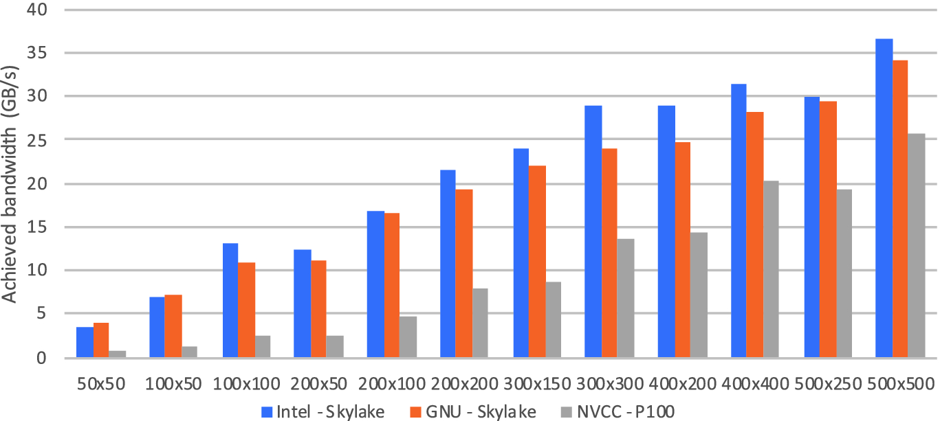
Most of our results show performance based on timing the purely computational part of the code, which does not include start-up costs such as reading data from a file, or even the data layout transformation (where applicable) - this is discussed separately at the end of Sect. 4.3.

../images/491247_1_En_12_Chapter/491247_1_En_12_Fig4_HTML.png — Fig. 4.
Bandwidth on Skylake CPU and P100 GPU when solving a single system

4.3 Results

First, we discuss baseline results that do not use the new API of OPS, and solve only a single system. The results are shown in Fig. 4; due to the small size of individual systems, utilisation is low, but increases steadily with larger systems. On the CPU, it does reach 58% of peak bandwidth at the largest problem, but on the P100 GPU these sizes are still far too small to efficiently use the device. For completeness, here we show performance achieved with both the Intel and the GNU compilers – the latter is 5–15% slower, and this difference is observed on later tests as well, which we omit for space reasons.

Next, we discuss the effect of optimisations at the other extreme, having 1000 systems. Results are shown in Fig. 5. The two basic strategies use flat OpenMP parallelism - here each ops_par_loop is extended with an extra loop over the different systems and parallelised over the outermost loop using OpenMP. The two variants of this scheme are when data is laid out in a way so values from subsequent systems are in the last dimension (Dim 2 - $x\_size \times y\_size \times \#systems$ ), or in the first dimension (Dim 0 - $\#systems \times x\_size \times y\_size$ ). Results clearly show the advantage of the Dim 2 layout, which consistently achieves 45–50 GB/s, or 72–80% of peak, as opposed to the 35–40 GB/s achieved by the Dim 0 layout. This is in part due to the Intel compilers having vectorised all the loops regardless of layout, and the loss in parallel efficiency when executing remainder loops being negligible.

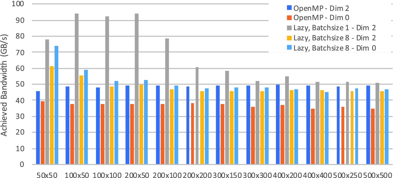
../images/491247_1_En_12_Chapter/491247_1_En_12_Fig5_HTML.png — Fig. 5.
Achieved bandwidth on the Skylake CPU when using different optimisations, solving 1000 systems

When enabling execution schedule transformations, relying on the lazy execution functionality of OPS, we can specify a Batchsize parameter - the number of systems to be solved together by a single thread. There are then combined with various data layouts, the two that are applicable here is the original Dim 2 layout, and the hybrid batched layout in Dim 0 ( $batch\_size \times x\_size \times y\_size \times \#systems/batch\_size$ ) - the flat Dim 0 layout causes non-contiguous memory accesses when solving groups of systems separately, and performs poorly, therefore it is not shown in this figure.

Two obvious choices for the Batchsize parameter are 1 - where the Dim 2 and hybrid Dim 0 layouts are actually the same, and a Batchsize that matches the vector length of the CPU, which in this case is 8 (512 bit vector length with 64 bit doubles). For the Dim 2 layout smaller batch sizes may be useful to mitigate any overheads in executing an ops_par_loop on a given system. For the Dim 0 layout having fewer systems in a batch would result in the underutilisation of vector units, because the innermost loop (which is being vectorised) is over different systems.

For our application, which has a considerable memory footprint for each system, and is primarily bandwidth-limited, the performance of these combinations is driven by how efficiently they can use the cache. At the largest problems it is clear, that not even a single system fits in cache, therefore the performance is bound by DDR4 bandwidth, and the different approaches are within 10% of each other - the lazy execution variant is the fastest due to having fewer synchronisations than the flat OpenMP version. At smaller problem sizes however, the Batchsize = 1 version performs the best, achieving over 90 GB/s, well above the DDR4 bandwidth; this is due to the data for a single system still fitting in cache. The memory footprint of individual systems is shown in Table 1 - considering that on this CPU, each core has approximately 2.3 MB of L2+L3 cache, the drop in performance above system sizes of $200\times 50$ matches the cache capacity. At the smallest problem size, the caching effect is still observable on the Batchsize = 8 versions (8 systems of size $50\times 50$ have a memory footprint of 3.4 MB), but performance quickly falls below the DDR4 bandwidth when moving to larger problems. It should also be noted, that at Batchsize = 8, the Dim 0 layout always outperforms the Dim 2 layout, thanks to more efficient vectorisation. This suggests that on applications which have fewer data per grid point, this strategy may perform the best.

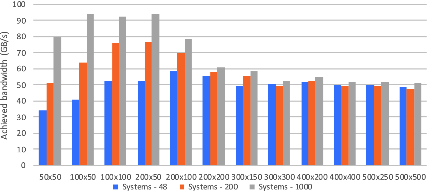
The number of systems to be solved is also an important factor to performance. Figure 6 shows the best performance out of the various optimisation options above, when running with 48, 200, or 1000 systems - system counts in-between are omitted from this figure as the behaviour is near-linear. Performance is bound by DDR4 bandwidth at larger problem sizes even at low system counts. It can be clearly observed that at smaller sizes, the larger the system count, the better the performance - in large part due to better load balance across different threads.

../images/491247_1_En_12_Chapter/491247_1_En_12_Fig6_HTML.png — Fig. 6.
Achieved bandwidth on the Skylake CPU when solving different numbers of systems

Finally, we evaluate performance on an NVIDIA Tesla P100 GPU. Here the range of options in terms of execution schedule and data layout transformations are more limited - cache locality cannot be reasonably exploited between subsequent CUDA kernel launches. This leaves us with the two layouts where the batching dimension is either the first or the last one (denoted as Dim 0 or Dim 2). However, the tridiagonal solver library exposes a number of algorithmic options for solving in the contiguous (X) dimension. There are no such options for solving in the Y or Z directions, as data accesses are naturally coalesced when adjacent threads solve adjacent systems. Figure 7 shows the results - Trid #0–4 denote the different X solve algorithms. While at smaller problem sizes, performance is affected by underutilisation, performance quickly reaches the 270–300 GB/s levels (50–55% of peak) for the two fastest options; when batching in Dim 0, and when using the Hybrid Thomas-PCR tridiagonal solver algorithm with register shuffles during the X solves for the Dim 2 layout.

../images/491247_1_En_12_Chapter/491247_1_En_12_Fig7_HTML.png — Fig. 7.
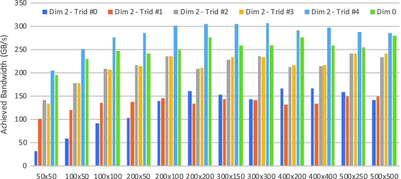
Achieved bandwidth on the P100 GPU when using different optimisations, solving 1000 systems

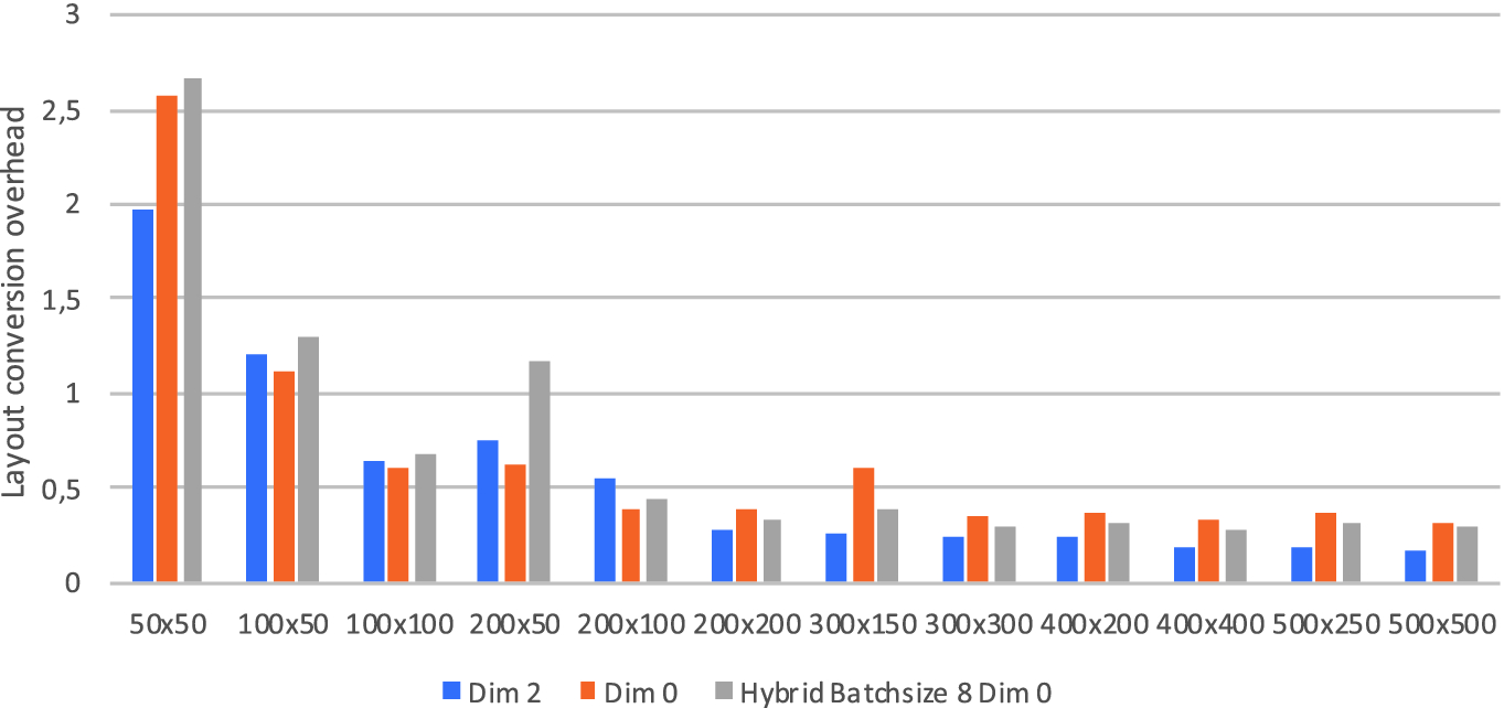
../images/491247_1_En_12_Chapter/491247_1_En_12_Fig8_HTML.png — Fig. 8.
Overhead of data layout conversion relative to the cost of a single time iteration, when using 200 systems.

The data layout transformations in particular have non-negligible overheads - OPS usually makes a copy of the user-supplied data even when no transformation is necessary to e.g. pad data in the X direction to a multiple of the cache line length. This transformation is parallelised by OPS using OpenMP, and its overhead is reported. Here, we show the overhead in relative terms compared to the time it takes to execute a single time iteration (for our tests we execute 10 time iterations). Figure 8 shows the overhead of the conversion from the default Dim 2 layout as the user provides the input, when using 200 systems - relative to the cost of a single time iteration. Clearly, the larger the system size the less the overhead, and it stabilises around the 0.25–0.35 time iteration cost. Conversion to Dim 0, or the hybrid layout is inevitably less efficient because of the strided memory accesses when writing data.

5 Conclusions

In this paper we have considered the challenge of performing the same calculations on multiple independent systems on various hardware platforms. We discussed a number of data layout options, as well as execution schedules, and integrated these into the OPS library. Our work allows users to trivially extend their single-system code to operate on multiple systems, and gives them the ability to easily switch between data layouts and execution schedules, thereby granting productivity. We have evaluated our work on state-of-the art Intel CPUs and NVIDIA GPUs, and an industrially representative financial application. Our experiments demonstrate that a high fraction of peak throughput can be achieved - delivering performance portability.

Acknowledgements

István Reguly was supported by the János Bolyai Research Scholarship of the Hungarian Academy of Sciences. Project no. PD 124905 has been implemented with the support provided from the National Research, Development and Innovation Fund of Hungary, financed under the PD_17 funding scheme. Supported by the ÚNKP-18-4-PPKE-18 new National Excellence Program of the Ministry of Human Capacities.

References

1.
OPS Library (2014). https://github.com/OP-DSL/OPS
2.
Bauer, M., Treichler, S., Slaughter, E., Aiken, A.: Legion: expressing locality and independence with logical regions. In: SC’12: Proceedings of the International Conference on High Performance Computing, Networking, Storage and Analysis, pp. 1–11. IEEE (2012)
3.
Carter Edwards, H., Trott, C.R., Sunderland, D.: Kokkos. J. Parallel Distrib. Comput. 74(12), 3202–3216 (2014). https://doi.org/10.1016/j.jpdc.2014.07.003Crossref
4.
Chandra, R., Dagum, L., Kohr, D., Menon, R., Maydan, D., McDonald, J.: Parallel Programming in OpenMP. Morgan Kaufmann, San Francisco (2001)
5.
Deakin, T., Price, J., Martineau, M., McIntosh-Smith, S.: Evaluating attainable memory bandwidth of parallel programming models via babelstream. Int. J. Comput. Sci. Eng. 17(3), 247–262 (2018)
6.
Gropp, W., Thakur, R., Lusk, E.: Using MPI-2: Advanced Features of the Message Passing Interface. MIT press, Cambridge (1999)Crossref
7.
Hornung, R.D., Keasler, J.A.: The RAJA portability layer: Overview and status. Technical report, Lawrence Livermore National Lab. (LLNL) (9 2014). https://doi.org/10.2172/1169830
8.
Hundsdorfer, W.: Accuracy and stability of splitting with stabilizing corrections. Appl. Numer. Math. 42(1–3), 213–233 (2002)MathSciNetCrossref
9.
In’t Hout, K., Welfert, B.: Stability of adi schemes applied to convection-diffusion equations with mixed derivative terms. Appl. Numer. Math. 57(1), 19–35 (2007)MathSciNetCrossref
10.
In’t Hout, K., Welfert, B.: Unconditional stability of second-order adi schemes applied to multi-dimensional diffusion equations with mixed derivative terms. Appl. Numer. Math. 59(3–4), 677–692 (2009)MathSciNetCrossref
11.
Jammy, S.P., Mudalige, G.R., Reguly, I.Z., Sandham, N.D., Giles, M.: Block-structured compressible navier-stokes solution using the ops high-level abstraction. Int. J. Comput. Fluid Dyn. 30(6), 450–454 (2016). https://doi.org/10.1080/10618562.2016.1243663MathSciNetCrossref
12.
Kronawitter, S., Kuckuk, S., Köstler, H., Lengauer, C.: Automatic data layout transformations in the exastencils code generator. Mod. Phys. Lett. A 28(03), 1850009 (2018)MathSciNet
13.
László, E., Giles, M., Appleyard, J.: Manycore algorithms for batch scalar and block tridiagonal solvers. ACM Trans. Math. Softw. 42(4), 31:1–31:36 (2016). https://doi.org/10.1145/2830568. http://doi.acm.org/10.1145/2830568MathSciNetCrossrefzbMATH
14.
MacNeice, P., Olson, K.M., Mobarry, C., De Fainchtein, R., Packer, C.: Paramesh: a parallel adaptive mesh refinement community toolkit. Comput. Phys. Commun. 126(3), 330–354 (2000)Crossref
15.
Mudalige, G.R., Reguly, I.Z., Giles, M.B., Mallinson, A.C., Gaudin, W.P., Herdman, J.A.: Performance analysis of a high-level abstractions-based hydrocode on future computing systems. In: Jarvis, S.A., Wright, S.A., Hammond, S.D. (eds.) PMBS 2014. LNCS, vol. 8966, pp. 85–104. Springer, Cham (2015). https://doi.org/10.1007/978-3-319-17248-4_5Crossref
16.
Nath, R., Tomov, S., Dongarra, J.: An improved magma gemm for fermi graphics processing units. Int. J. High Perform. Comput. Appl. 24(4), 511–515 (2010)Crossref
17.
Nvidia, C.: Programming guide (2010)
18.
Reguly, I.Z., Mudalige, G.R., Giles, M.B.: Loop tiling in large-scale stencil codes at run-time with OPS. IEEE Trans. Parallel Distrib. Syst. 29(4), 873–886 (2018). https://doi.org/10.1109/TPDS.2017.2778161Crossref
19.
Reguly, I.Z., Mudalige, G.R., Giles, M.B., Curran, D., McIntosh-Smith, S.: The ops domain specific abstraction for multi-block structured grid computations. In: 2014 Fourth International Workshop on Domain-Specific Languages and High-Level Frameworks for High Performance Computing, pp. 58–67, November 2014. https://doi.org/10.1109/WOLFHPC.2014.7
20.
Siklosi, B., Reguly, I.Z., Mudalige, G.R.: Heterogeneous cpu-gpu execution of stencil applications. In: 2018 IEEE/ACM International Workshop on Performance, Portability and Productivity in HPC (P3HPC), pp. 71–80, November 2018. https://doi.org/10.1109/P3HPC.2018.00010
21.
Stone, J.E., Gohara, D., Shi, G.: Opencl: a parallel programming standard for heterogeneous computing systems. Comput. Sci. Eng. 12(3), 66 (2010)Crossref
22.
Tataru, G., Fisher, T.: Stochastic local volatility. Quantitative Development Group, Bloomberg Version 1(February 5) (2010)
23.
Verwer, J.G., Spee, E.J., Blom, J.G., Hundsdorfer, W.: A second-order rosenbrock method applied to photochemical dispersion problems. SIAM J. Sci. Comput. 20(4), 1456–1480 (1999)MathSciNetCrossref
24.
Wang, H.: A parallel method for tridiagonal equations. ACM Trans. Math. Software (TOMS) 7(2), 170–183 (1981)MathSciNetCrossref
25.
Wyns, M., Du Toit, J.: A finite volume-alternating direction implicit approach for the calibration of stochastic local volatility models. Int. J. Comput. Math. 94(11), 2239–2267 (2017)MathSciNetCrossref
26.
Zingale, M., et al.: Meeting the challenges of modeling astrophysical thermonuclear explosions: castro, maestro, and the amrex astrophysics suite. In: Journal of Physics: Conference Series, vol. 1031, p. 012024. IOP Publishing (2018)