1 Introduction
The turbulent motion of fluid flows poses some of the most difficult and fundamental problems in classical physics as it is a complex, strongly non-linear, multi-scale phenomenon [36]. A general challenge in turbulence research is to predict the statistics of fluctuating velocity and scalar fields and develop models for a precise statistical prediction of these fields even in scale-resolved simulations [21, 34].
Large-eddy simulation (LES) is known to be a suitable modeling approach for turbulent flows and solves for the larger, flow-dependent scales of the flow by modeling all scales below a particular filter width [15, 28]. It is assumed that the smaller, unresolved scales reveal certain universal features and decouple from the larger non-universal scales. As a consequence, models for LES can be built from relatively simple, semi-empirical algebraic relations that are oftentimes based solely on dimensional arguments [40]. One approach to develop and test such models is to perform fully resolved direct numerical simulations (DNSs), filter the resulting data with a given filter kernel, and find functional relations between the DNS results and the filtered data. The objective of the present work is to move beyond simple algebraic models for LES and use a data-driven approach with deep learning (DL) for modeling and reconstructing subfilter statistics for turbulent flows.
DL has gained immense interests from various industries and research groups in the age of big data. Prominent applications of DL include image processing [8, 17, 42, 43], voice recognition [18], or website customization [24]. Reasons for that are the continued growth of computational power (especially GPUs) and the availability of exceptionally large labeled experimental data sets. Also in the field of fluid mechanics and especially turbulence research, data-driven methods and DL have become more popular over the last years. However, often the applications are limited by either using only simple networks or small, artificial datasets.
Parish and Duraisamy [33] used an approach called field inversion and machine learning (FIML), which moves beyond parameter calibration and uses data to directly infer information about the functional form of model discrepancies. They applied their approach to turbulent channel flows. Srinivasan et al. [41] assessed the capabilities of neural networks to predict temporally evolving turbulent flows and concluded that long short-term memory (LSTM) networks perform better than multi-layer perceptron (MLP) approaches. Ling et al. [29] also presented a method using deep neural networks to learn a model for the Reynolds stress anisotropy tensor from high-fidelity simulations and experimental data. The Reynolds stress anisotropy predictions were found to be more accurate than conventional Reynolds-averaged Navier-Stokes (RANS) models, however the network could not perfectly reproduce the DNS results. Milano and Koumoutsakos [31] modeled the near-wall region of turbulent flows. Lapeyre et al. [25] and Beck et al. [4] have documented the possibility of using ML in designing subgrid-scale models for LES. Maulik and San [30] presented their use of a single-layer feedforward artificial neural network (ANN) architecture trained through a supervised learning approach for the deconvolution of flow variables from their coarse-grained computations such as those encountered in LES. The subfilter-scale content recovery was benchmarked against several popular structural closure modeling strategies. Bode et al. [5] studied the accuracy of various network architectures for predicting statistics of turbulent flows. Machine learning (ML) and DL have also been applied to flow control [14, 27], development of low-dimensional models [38], generation of inflow conditions [11], or structure identification in two-dimensional (2-D) decaying turbulence [19]. Kutz [23] summarized more applications of DL in the field of fluid dynamics.
This work focuses on two different approaches in the context of data-driven turbulence modeling with DL: regression and reconstruction. In the regression part, a supervised learning method is used to predict closure terms in the context of LES modeling based on filtered quantities. Simple ANNs are employed to predict, for example, the turbulent viscosity or the scalar dissipation rate. In the reconstruction part, a generative adversarial network (GAN) approach is followed to reconstruct fully-resolved turbulence fields from filtered data. Results with respect to different network architectures and different quantities are discussed here. Furthermore, DL based on 3-D scientific data differs from DL on images not only in terms of the size of total data but also in the size of a single realization used for training. The size of scientific data can easily be in the order of hundreds of terabytes while training is traditionally performed with much smaller data. Therefore, DL on scientific data is often not possible without the usage of supercomputers and corresponding high performance computing (HPC) approaches. These computing aspects are also discussed in this work.
The remainder of this article is organized as follows. Section 2 describes the used datasets. In Sect. 3, details about the regression and reconstruction methodologies are given, and results are discussed. Challenges with respect to computational aspects are addressed in Sect. 4. The paper finishes with conclusions.
2 Dataset Description
The training and reconstruction is based on data obtained from high-fidelity homogeneous isotropic forced turbulence simulations [12, 13] in this work. The data was generated by DNSs of the incompressible Navier-Stokes equations (NSEs) in a triply periodic cube with size  and
and  collocation points. Moreover, advection-diffusion equations of passive scalars were solved, which were used for tracking species or mixture factions. Turbulence was kept in a statistically steady state by a large-scale stochastic forcing scheme [10], whereas the passive scalars were forced by an imposed uniform mean gradient. The governing equations were solved by an accurate pseudo-spectral approach with integrating factor technique. A pseudo-spectral approach with integrating factor technique was used for accuracy. For efficiency, the non-linear transport term of the NSEs was computed in physical space, and a truncation technique with a smooth spectral filter was applied to reduce aliasing errors. The library P3DFFT was used for the spatial decomposition and to perform the fast Fourier transform. The code employs a hybrid MPI/OpenMP parallelization and reveals a nearly linear scaling up to two million threads.
 , for example defined based on the Taylor length scale
  as
as
 is the kinematic viscosity and
  is the root-mean-square deviation of the velocity vector
  .
.  is defined as
 to the DNS data, i.e.

 as the magnitude of the wavenumber vector
  , is used. The Gaussian filter kernel is local in both spectral and real space and avoids erroneous fluctuations in the filtered fields. The cut-off wavenumber
  is related to the filter-width
  by
by
 , which corresponds to a length scale at the end of the restricted scaling range. Characteristic quantities of the DNSs and the filtered data are given in Table 1. Here,
  denotes the ensemble-averaged turbulent kinetic energy,
  the ensemble-averaged dissipation rate of turbulent kinetic energy, and
  the ensemble-averaged dissipation rate of scalar variance. All quantities in this work are arbitrarily normalized without loss of generality.
Characteristic properties of the DNSs and the filtered velocity and scalar field.
Case A | Case B | |
|---|---|---|
| 9.67 | 10.93 |
| 9.19 | 10.36 |
| 10.69 | 13.06 |
| 8.62 | 10.11 |
| 3.30 | 6.59 |
| 2.16 | 4.11 |
| 42.7 | 43.7 |
3 Modeling
This section describes the regression and reconstruction approaches by showing results for two network architectures. All networks were implemented using the Keras API [1] built on the TensorFlow [2] backend.
3.1 Regression
 modeled as
 is a model constant,
  is the filter width, and
  is the filtered rate of strain tensor defined as
 being the del operator. Furthermore, the prediction of turbulent mixing requires an accurate prediction of the mean scalar dissipation rate
  , which is the sink term in the transport equation of the mean scalar variance
  . Here, the local instantaneous scalar dissipation rate is defined as
 denotes the transported scalar quantity, and D is the molecular diffusivity. All scalars were shifted to zero mean in this work. The mean scalar dissipation rate is related to the scalar variance spectrum
  by
by
 . As these scales are not available in coarse-grained fields or LES, an accurate modeling of
  is necessary.
In the context of LES modeling, regression evaluated with neural network architectures can be used to obtain optimal predictions of subgrid quantities or contributions based on the incomplete information resolved in the LES. One example is to train a DL network with filtered DNS quantities as input and the corresponding DNS quantities as ‘label’ to learn the relation between the quantities resolved in LESs and their subgrid contributions. In the following subsections, this will be shown with simple feedforward ANNs. Unlike classical linear or logistic regression models, regression through neural networks can represent more complex functions by data manipulations through dense layers. The number of layers and the number of nodes in each layer can be varied to obtain optimal networks and results [29]. Activation functions in each layer can be used to add non-linearity to the regression model, and a dropout layer can be added for regularization, so that certain nodes are ignored during training to reduce overfitting or high variance. In the next subsection, regression is used to reproduce the turbulent viscosity model introduced in Eq. (6), which will show that simple DL networks are able to learn from the considered DNS data. Afterwards, several regression models for the scalar dissipation rate are evaluated. All cases were run for 7000 epochs, and the evolutions of the loss functions are shown to evaluate the convergence of the training.
 Prediction Using
  : As network validation, a single input value, single output value mapping was implemented relating
  and
and  by means of a 3-layer neural network as shown in Fig. 1. Figure 2 compares the modeled
  , obtained from Eq. (6), with the prediction from the network. The good collapse of both curves for all values of
  validates that the network is able to learn simple relations as given by Eq. (6).
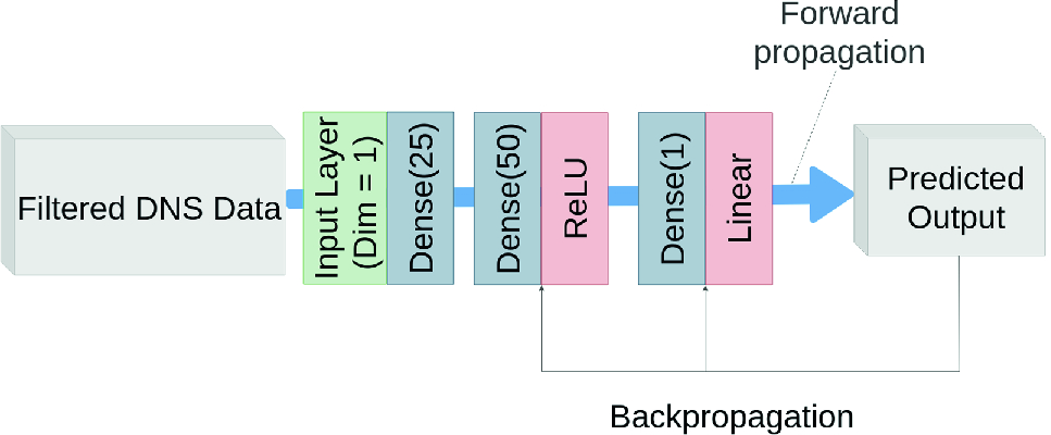
Sketch of the network for  prediction.
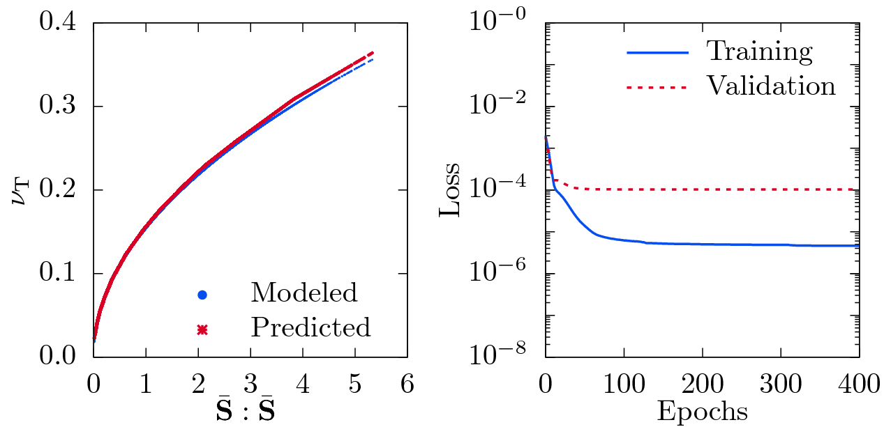
Visualization of the modeled and DL-predicted turbulent viscosity  using the double inner product of two filtered rate of strain tensors
  as input (left) and the corresponding loss as function of number of epochs (right).
 Prediction Using
  : After validating the network with predicting
  , feedforward networks are used to predict the resolved scalar dissipation rate
  . The accuracy of the prediction is strongly affected by the considered input variables and the network architecture and parameters. It was found that the 3-layer network shown in Fig. 1, which works well for predicting
  , leads to inaccuracies for predictions of the resolved scalar dissipation rate. The accuracy could be improved by switching to a 5-layer network architecture as visualized in Fig. 3. Even more layers did not improve the prediction accuracy further, and therefore, the following plots are based on training with the 5-layer network.
Sketch of the network for  prediction.
 as only input to the network, which is equal to the filtered scalar fluctuations
  here. The obtained results are shown in Fig. 4, and good correlation between the DNS and the DL-predicted values of
  can be seen. Note that the negative values of the scalar dissipation rate result from a centering and rescaling of the scalar dissipation rate fields indicated by the tilde symbol. The good correlation implies that the network is able to learn the derivatives of
  (cf. Eq. (8)), even though no convolutional layer was used here. Moreover, the probability density function (PDF) of
  is plotted in Fig. 5 to further assess the accuracy of the prediction. The scalar dissipation rate is a very intermittent quantity, which implies the presence of very strong but very rare events. These strong events are characteristic features of turbulence and play an important role for small-scale mixing or turbulent combustion. Comparing the PDFs of the DNS and DL-predicted scalar dissipation rates indicates that the dense fully connected neural network is able to reproduce the PDF of
  with moderate accuracy as clear deviations are seen in the logarithmic plot.
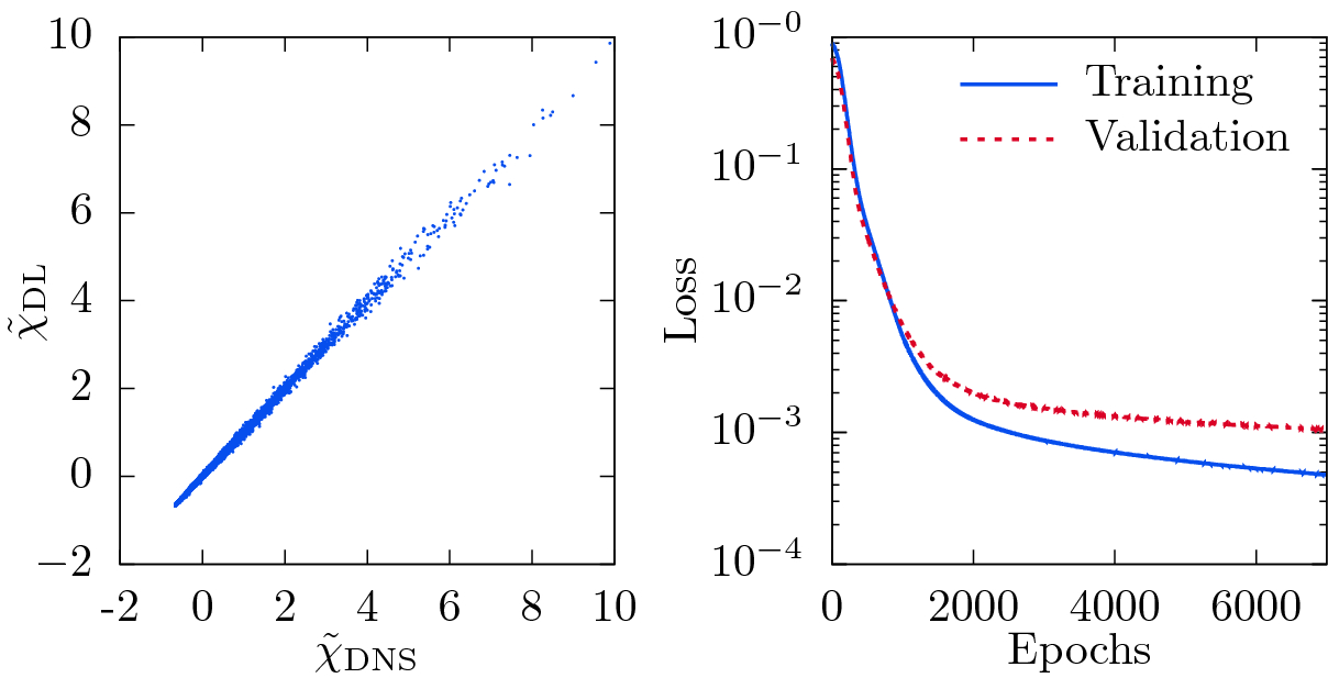
Visualization of the correlation between DNS and DL-predicted rescaled scalar dissipation rate  using the filtered passive scalar
  as input (left) and the corresponding loss as function of number of epochs (right).
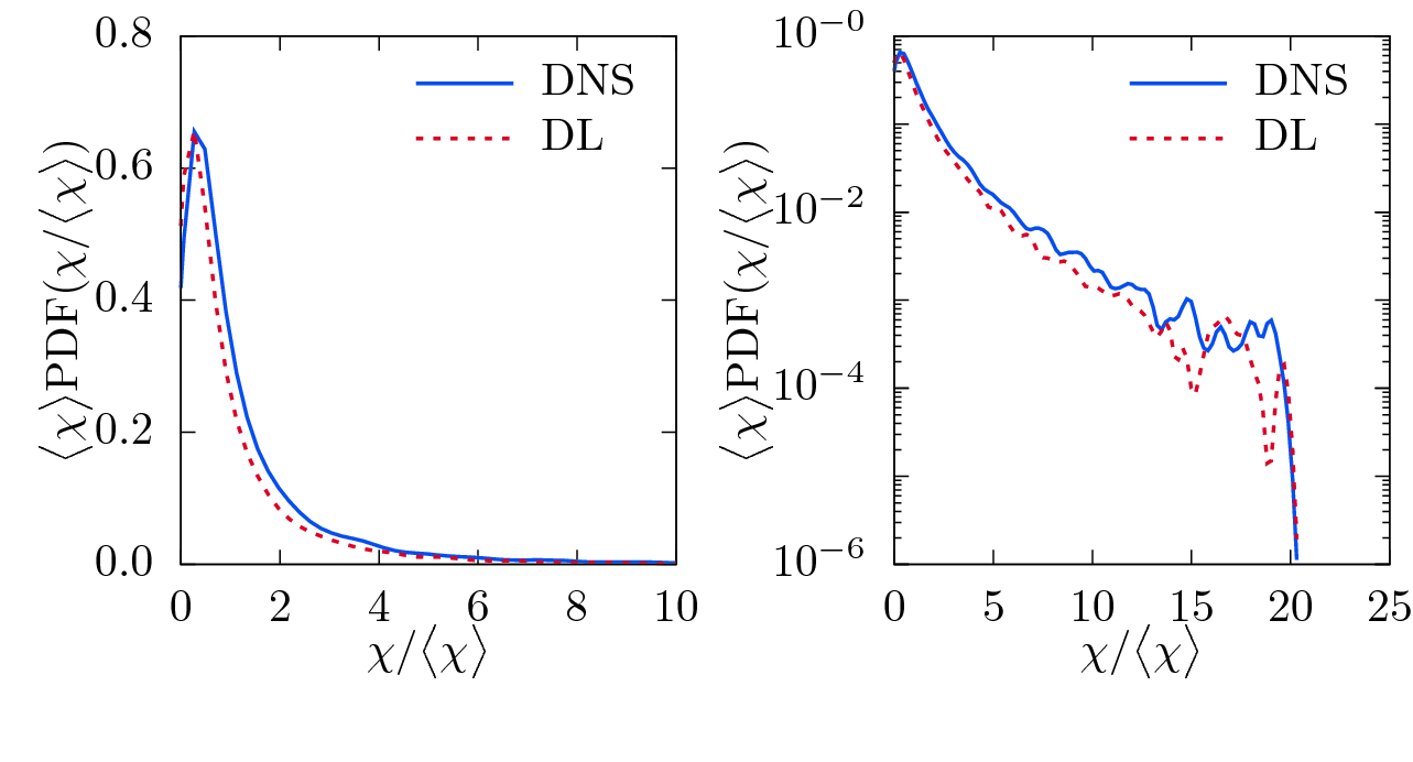
Visualization of the normalized PDF of the DNS and DL-predicted scalar dissipation rate  with linear (left) and logarithmic (right) ordinate for the network with filtered passive scalar
  as input.
 Prediction Using
  and
and  : Classical models in turbulence propose that the mean scalar dissipation rate
  depends on the scalar variance
  and a characteristic time-scale
  , i.e.
 is a constant.
  is usually chosen as an integral time-scale and can be defined as
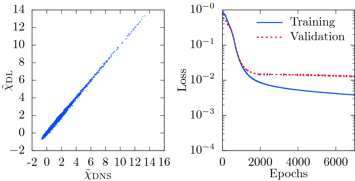
Visualization of the correlation between DNS and DL-predicted rescaled scalar dissipation rate  using the filtered passive scalar
  and filtered energy dissipation rate
  as inputs (left) and the corresponding loss as function of number of epochs (right).
 on the characteristic time-scale
  , which leads to the observed deviations. Following Overholt and Pope [32] and motivated by Eq. (10), the input for the network predicting the scalar dissipation rate
  is extended by the resolved energy dissipation rate
  , defined as

 provides additional information about the local time scales of turbulence to the network.
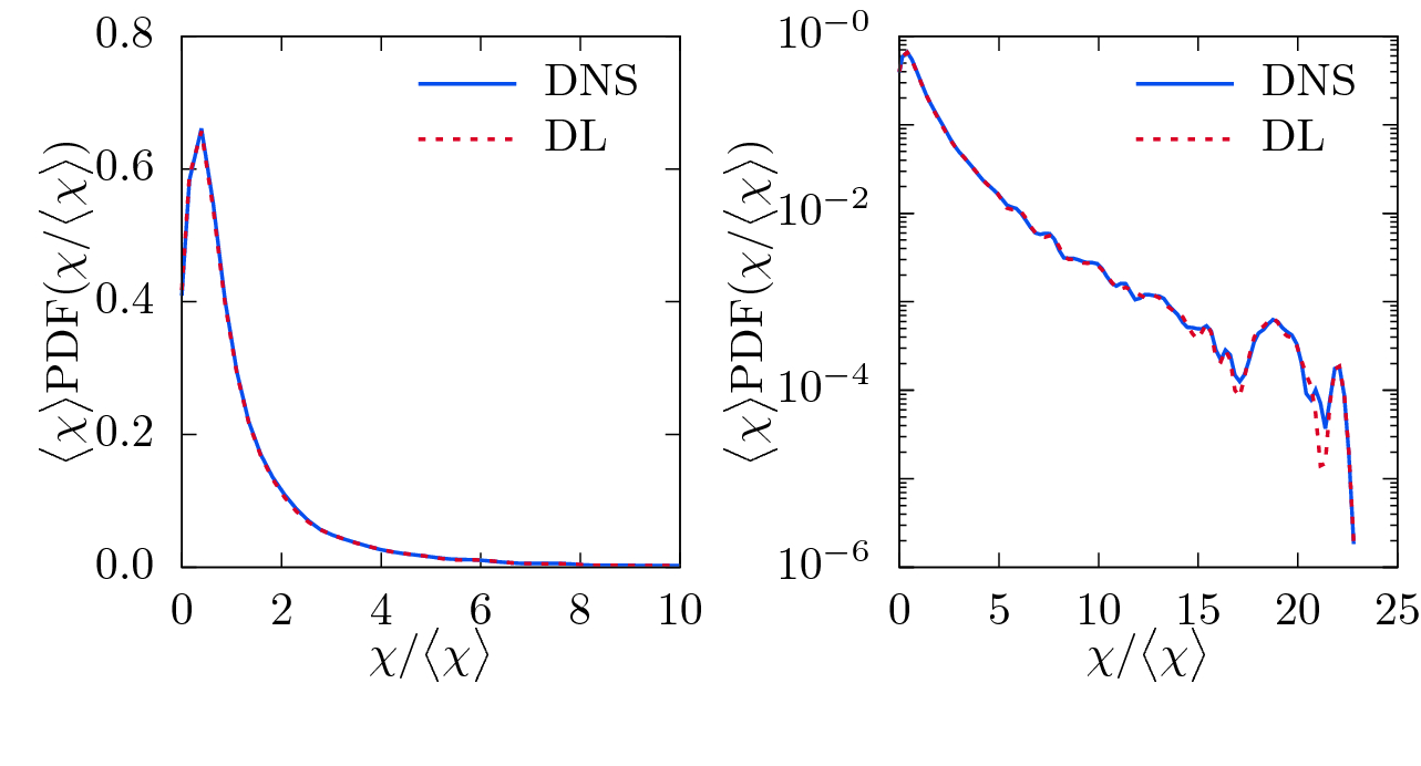
Visualization of the normalized PDF of the DNS and DL-predicted scalar dissipation rate  with linear (left) and logarithmic (right) ordinate for the network with filtered passive scalar
  and filtered energy dissipation rate
  as inputs.
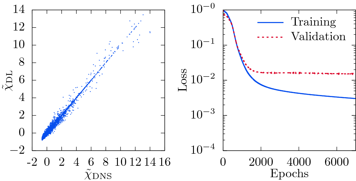
Visualization of the correlation between DNS and DL-predicted rescaled scalar dissipation rate  using the filtered passive scalar
  and filtered velocity
  as inputs (left) and the corresponding loss as function of number of epochs (right).
 Prediction Using
  and
and  : After successfully predicting the scalar dissipation rate with good accuracy, it is tested whether the network is also able to extract the time scale information contained in the filtered energy dissipation rate from the filtered velocity
  , which is used to compute the filtered energy dissipation rate (cf. Eqs. (7) and (13)). Therefore, the network inputs are changed to
  and
and  , and the results are shown in Figs. 8 and 9. It can be seen that the prediction quality is worse compared to Figs. 6 and 7, which indicates that the network is not fully able to learn the tensor operations performed in Eqs. (7) and (13). Interestingly, the result is also worse than the results shown in Figs. 4 and 5, which might be due to overfitting.
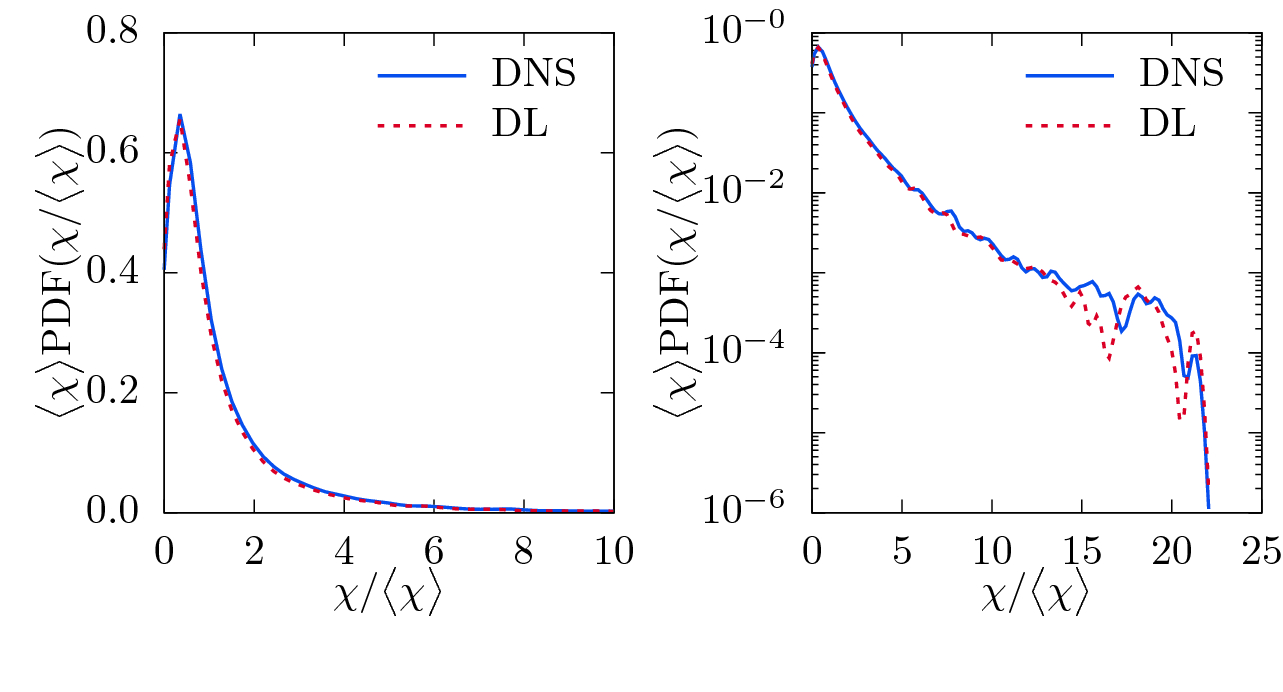
Visualization of the normalized PDF of the DNS and DL-predicted scalar dissipation rate  with linear (left) and logarithmic (right) ordinate for the network with filtered passive scalar
  and filtered velocity
  as inputs.
3.2 Reconstruction
Reconstructing the fully-resolved flow from large-scale or coarse-grained data has significant applications in various domains. For example, particle image velocimetry (PIV) measurements can only resolve information on large scales due to limited spatial resolution [7]. Similarly, LES is widely used for weather predictions [35], where resolving the small-scale information is prohibitively expensive. The reconstruction of subgrid information with deep learning networks is a promising approach to link the large-scale results obtained from experiments or filtered equations to the actual flow fields.
In this subsection, a GAN-approach is used to reconstruct fully-resolved 3-D velocity fields from filtered data. With these fields, the filtered NSEs can be closed.
Network Motivation: The DL network used for reconstruction in this work is inspired by the enhanced super-resolution GAN (ESRGAN) introduced by Wang et al. [43] for reconstructing filtered features in 2-D images, which is a leading DL-approach in the field of single image super-resolution (SISR). A pioneering work in the field of SISR was the SRCNN proposed by Dong et al. [8]. The general concept of GANs was presented by Goodfellow et al. [16]. A GAN is composed of two models, a generator that captures the data distribution and generates new data, and a discriminator that learns to distinguish whether a sample stems from the original data distribution (genuine) or the generator (fake). During training, the generator learns to produce samples that are indistinguishable for the discriminator, while the discriminator learns to more accurately judge the genuineness. For better perceptual similarities, Ledig et al. [26] introduced the SRGAN, which takes the perceptual loss into consideration while evaluating the cost function. Instead of calculating the root-mean-square error (RMSE) in pixel space, the content loss is implied by calculating the RMSE in VGG19 [39] feature space, i.e. the VGG loss. This grants the SR-images produced by a SRGAN generator satisfying perceptual similarity to the original image as well as optimized recovery of the high frequency details. However, SRGAN produced hallucinated details accompanied with unpleasant artifacts in the images [43]. Hence, Wang et al. proposed the Enhanced SRGAN (ESRGAN) to alleviate such problems by building a residual-in-residual dense block (RRDB) into the SRGAN generator and adopting the idea of relativistic GAN [20].
The ESRGAN has been extended to a turbulence super-resolution GAN (TSRGAN) for this work, as shown in Fig. 10. The TSRGAN is able to deal with 3-D subboxes of the filtered DNS data (scalar and vector fields) as input and employs physics-based loss functions for training of the network. Validation results of the TSRGAN trained with 800 images from the DIV2K archive [3] over 50000 epochs are presented in Fig. 11. Besides the good quality of 2-D reconstruction on images, also the similarity in terms of tensor operations seems to make the TSRGAN a promising candidate for reconstruction of filtered flow data. A filter operation can be seen as convolution, and the network architecture of the TSRGAN heavily relies on convolutional layers.
Loss Function: The perceptual loss proposed for the ESRGAN based on VGG-feature space is apparently not as suitable for the turbulence data, as the geometrical features from VGG19 are not representative for turbulent flows. Hence, a new formulation for the cost function was developed inspired by physical flow constraints.

 , and
, and  being coefficients weighting the different loss term contributions.
  is the ‘realistic average’ discriminator/generator loss, which is the accuracy feedback between discriminator and generator as given by Wang et al. [43]. The pixel loss
  is defined as

 as number of all samples, i.e. the total number of grid points of the reconstructed field. If the MSE operator is applied on tensors including vectors, it is applied to all elements separately. Afterwards the resulting tensor is mapped into a scalar using the 1-norm. The gradient loss
  is defined as
 is the continuity loss, which enforces the continuity equation in the reconstructed field and reads
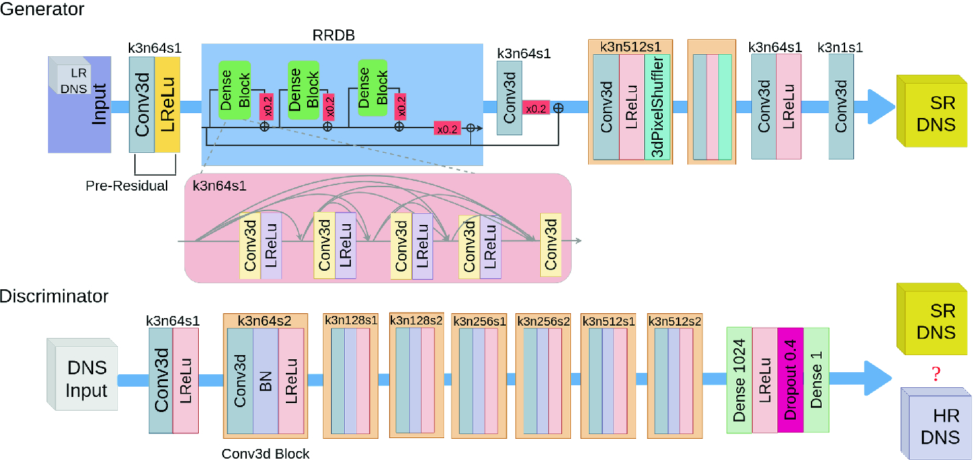
Sketch of the network used for the reconstruction.

Comparison of an original (left), bicubic interpolated (center), and TSRGAN-reconstructed image.
The original image is taken from the DIV2K archive [3].

 is the enstrophy. By definition, Q is a small-scale quantity, which is suitable to assess the turbulent motions in the dissipative range. The agreement between DNS and reconstructed data is good.
 is a statistical representation of the turbulent kinetic energy in wavenumber space. Different scales can be distinguished: the energy-containing range at small wavenumbers, the inertial subrange at intermediate wavenumbers, and the dissipative range at large wavenumbers. However, it is important to emphasize that a well defined scale-separation between small and large scales only exists at sufficiently high Reynolds numbers. When
  is known, the mean turbulent energy can be obtained by

 than on the filtered mean turbulent energy
  .
.
Comparison of 2-D slices of the filtered (left), DL-reconstructed (center), and DNS (right) data. Snapshots of the three elements of the velocity vector  are shown row-by-row.

Comparison of 2-D slices of turbulent kinetic energy k snapshots for filtered (left), DL-reconstructed (center), and DNS (right) data.
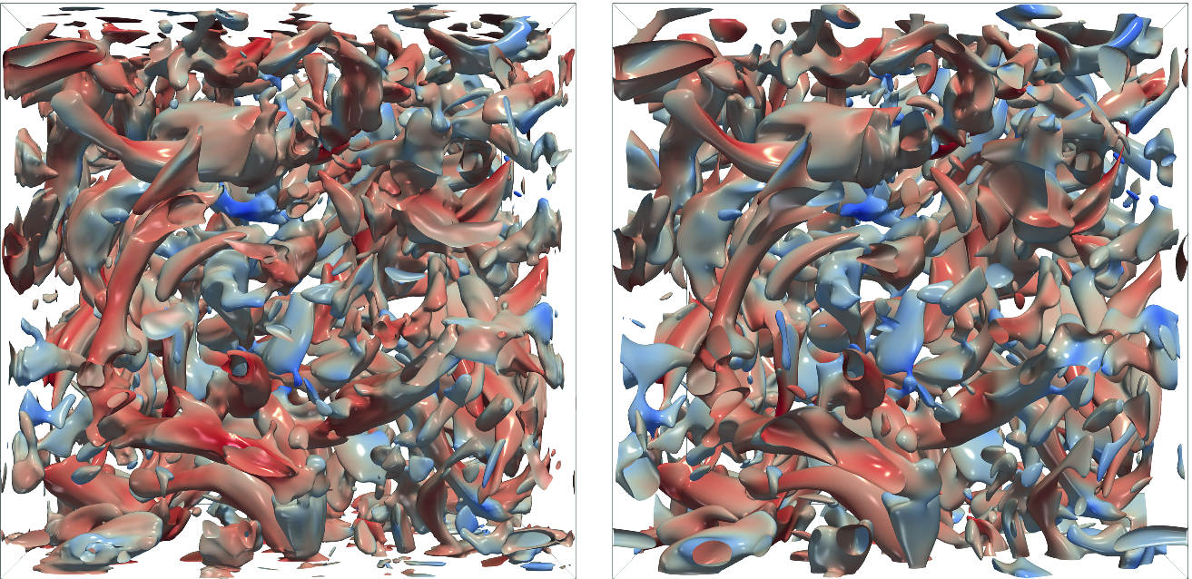
Comparison of the Q-criterion evaluated on the DL-reconstructed (left) and DNS (right) data.

Comparison of the energy spectra  evaluated on the DNS, DL-reconstructed, and filtered data.
4 Computing
Typically, the single node performance of DL training is very good due to the heavy use of linear algebra-based primitives and the optimization of current GPUs for tensor operations. This is especially true if state-of-the-art libraries, such as TensorFlow, which are highly optimized for GPU usage, are used, as in this work. However, HPC-DL is still challenging. A common way for parallelizing the training of DL networks is to replicate the network across ranks. Thus, each rank processes a different local batch of DNS data, and updates to the network are aggregated among ranks during each training step.
For transforming single-process TensorFlow entities into a data-parallel implementation, Horovod [37] was used, which adds allreduce operations into the back-propagation computation to average the computed gradients from each rank’s network. The local networks are updated by the ranks independently, which results in synchronous distributed training due to the use of gradients averaged across all ranks. Obviously, two main challenges are the communication of the information and I/O of data for this procedure. They are addressed separately in the next two subsections. All highly-parallel training for this work was performed on the Supercomputer JURECA at Jülich Supercomputing Centre (JSC), which features nodes equipped with two NVIDIA K80 GPUs (four visible devices per node). Finally, it was possible to train networks with up to 396.2 TFLOPS on JURECA.
4.1 Communication
Horovod uses the first rank as central scheduler for all Horovod operations, employing a dynamical reordering of allreduce operations in order to achieve consistency among all ranks and avoid deadlock due to the independent scheduling of all TensorFlow entities. With an increasing number of ranks, the central scheduler becomes more and more a communication bottleneck as it needs to handle all readiness messages of all other ranks. As a distribution of this scheduling load is not possible due to the required total order of the collective operations, a communication tree was employed in this work. It allows to use Horovod’s original scheduler but limits the message load due to the recursive broadcast.
4.2 I/O
As a large amount of DNS data is required for the training of the network, the data transfer to the GPUs is often a bottleneck as the file system - on JURECA GPFS is used - is not fast enough to feed the GPUs in a timely fashion. For this work, a similar strategy as suggested by Kurth et al. [22] was employed. Only a significant fraction of the overall data set was made accessible to each node for the distributed training setting. The locally available data were combined to a local batch in such a way that the set of samples for each rank was statistically similar to a batch selected from the entire data set. Technically, a distributed data staging system was used that first divided the data set into disjoint pieces to be read by each rank, before distributing copies of each file to other nodes by point-to-point MPI messages. This approach takes advantage of the high bandwidth of the InfiniBand network without increasing the load on the file system.
5 Conclusion
Two DL approaches for modeling of subgrid statistics are presented in this paper. It is shown that simple feedforward ANNs are able to learn subgrid statistics with good accuracy if appropriate inputs are chosen. Furthermore, ESRGAN is extended to TSRGAN and used to reconstruct fully-resolved 3-D velocity fields. Both the visual agreement and the statistical agreement are very good, which indicates that the TSRGAN is able to predict small-scale turbulence. Finally, the code framework used for learning was optimized to achieve 396.2 TFLOPS on the supercomputer JURECA.
Acknowledgment
The authors gratefully acknowledge the computing time granted for the project JHPC55 by the JARA-HPC Vergabegremium and provided on the JARA-HPC Partition part of the supercomputer JURECA at Forschungszentrum Jülich. Also financial support by the Cluster of Excellence “The Fuel Science Center”, which is funded by the Deutsche Forschungsgemeinschaft (DFG, German Research Foundation) under Germany’s Excellence Strategy – Exzellenzcluster 2186 “The Fuel Science Center” ID: 390919832, and from of the European Research Council (ERC) under the European Union’s Horizon 2020 research and innovation program under grant agreement No. 695747 is acknowledged. MG acknowledges financial support provided under the grant EMCO2RE. Furthermore, the authors want to thank Jenia Jitsev, Zeyu Lian, and Mayur Vikas Joshi for their help.


