© Springer Science+Business Media LLC 2018

Joseph I. Goldstein, Dale E. Newbury, Joseph R. Michael, Nicholas W.M. Ritchie, John Henry J. Scott and David C. JoyScanning Electron Microscopy and X-Ray Microanalysishttps://doi.org/10.1007/978-1-4939-6676-9_17

17. DTSA-II EDS Software

Joseph I. Goldstein¹ , Dale E. Newbury², Joseph R. Michael³, Nicholas W. M. Ritchie², John Henry J. Scott² and David C. Joy⁴

(1)

University of Massachusetts, Amherst, Massachusetts, USA

(2)

National Institute of Standards and Technology, Gaithersburg, Maryland, USA

(3)

Sandia National Laboratories, Albuquerque, New Mexico, USA

(4)

University of Tennessee, Knoxville, Tennessee, USA

 

17.1 Getting Started With NIST DTSA-II

17.1.1 Motivation

Reading about a new subject is good but there is nothing like doing to reinforce understanding. With this in mind, the authors of this textbook have designed a number of practical exercises that reinforce the book’s subject matter. Some of these exercises can be performed with software you have available to you—either instrument vendor software or a spreadsheet like MS Excel or LibreOffice/OpenOffice Calc. Other exercises require functionality which may not be present in all instrument vendor’s software. Regardless, it is much easier to explain an exercise when everyone is working with the same tools.

To ensure that everyone has the tools necessary to perform the exercises, we have developed the National Institute of Standards and Technology software called DTSA-II (Ritchie, 2009, 2010, 2011a, b, c, 2012, 2017a, b). NIST DTSA-II is quantitative X-ray microanalysis software designed with education and best practices in mind. Furthermore, as an output of the US Federal Government, it is not subject to copyright restrictions and freely available to all regardless of affiliation or nationality. From a practical perspective, this means that you can install and use DTSA-II on any suitable computer. You can give it to colleagues or students. You can use it at home, in your office, or in the lab. If you are so inclined, the source code is available to allow you to review the implementation or to enhance the tool for your own special purposes.

Exercises in the textbook will be designed around the capabilities of DTSA-II. Many will take advantage of the graphical user interface to manipulate and interrogate spectra. A number will take advantage of the command line scripting interface to access low-level data or to perform advanced operations.

17.1.2 Platform

NIST DTSA-II is written in the multi-platform run-time environment Java. This means that the same program runs on Microsoft Windows (XP, Vista, 7, 8.X, 10.X), Apple OS X 10.6+, and many flavors of Linux and UNIX. The run-time environment adjusts the look-and-feel of the application to be consistent with the standards for each operating system. For Windows, Linux, and UNIX, the main menu is part of the main application window. In OS X, the main menu is at the top of the primary screen.

To make installation as easy as possible on each environment, an installer has been developed which works on Windows, OS X, and Linux/UNIX. The installer verifies that an appropriate version of Java is available and place the executable and data files in a location that is consistent with operating system guidelines. Detailed installation instructions are available on the download site.

17.1.3 Overview

DTSA-II was designed around common user interface metaphors and should feel consistent with other programs on your operating system. It has a main menu which provides a handful of high-level interactions such as file access, processing, simulation, reporting, and help. Many of these menu items lead to “wizard-style” dialogs which take you step-by-step through some more complex operation like experiment design, spectrum quantification, or spectrum simulation. The goal is to make common operations as simple as possible.

Additional tools are often available through context sensitive menus. Each region on the DTSA-II main window provides different functionality. Within these regions, you are likely to want to perform various context sensitive operations. These operations are accesses through menus that are accessed by placing the mouse over the region and issuing a “right-button click” on Windows/Linux/UNIX or an Apple-Command key + mouse click on OS X. The context-sensitive menu items may perform operations immediately, or they may request additional information through dialog boxes.

On the main screen, the bottom half of window is three tabs—the Spectrum tab, the Report tab, and the Command tab. The spectrum tab is useful for investigating and manipulating spectra. The report tab provides a record of the work completed during this invocation of the program. Since the report is in HTML (Hypertext Markup Language) and stored by date, it is possible to review old reports either in DTSA-II or in a standard web browser. Some operating systems will index HTML documents making it easy to find old designs, analyses or simulations.

The final tab contains a command line interface. The command line interface implements a Python syntax scripting environment. Python is a popular, powerful and complete scripting language. Through Python it is possible (though not necessarily easy) to perform anything that can be done through the GUI. It is also possible to do a lot more. For example, the GUI makes available some common, useful geometries for performing Monte Carlo simulations of spectrum generation. Through scripting, it is possible to simulate arbitrary sample and detector geometries. Some of the examples in the text will involve scripting. These scripts will be installed with the software so they are readily available and so you can use these as the basis for your own custom scripts.

An important foundational concept in DTSA-II is the definition of an X-ray detector. The software comes with a “default detector” which represents a typical Si(Li) detector on a typical SEM. This detector will produce adequate results for many purposes. However, it is better and more useful if you create your own detector definition or definitions to reflect the design and performance of your detector(s) and SEM. You define your own detector using the “Preferences” dialog which is access through the “File → Preferences” main menu item. To select and activate your detector, you select it in the “Default Detector” drop down lists on the middle, left side of the main DTSA-II window on the “Spectrum Tab.”

17.1.4 Design

DTSA-II is, in many ways, much more like vendor software used to be. This has advantages and disadvantages. Over the years, vendors have simplified their software. They have removed many more advanced spectrum manipulation tools and they have streamlined their software to make getting an answer as straightforward as possible. If your goal is simply to collect a spectrum, press a button, and report a result, the vendor software is ideal. However, if you want to develop a more deep understanding of how spectrum analysis works, many vendors have buried the tools or removed them entirely. DTSA-II retains many of the advanced spectrum manipulation and interrogation tools.

DTSA-II is designed with Einstein’s suggestion about simplicity in mind: “Everything should be made as simple as possible, but not simpler.” DTSA-II was designed with the goal of making the most reliable and accurate means of quantification, standards-based quantification, as simple as possible, but not simpler. When there is a choice that might compromise reliability or accuracy for simplicity, reliability and accuracy wins out.

One such example is “auto-quant.” Most microanalysis software will automatically place peak markers on spectra. Unfortunately, these markers have time and time again been demonstrated to be reliable in many but far from all cases. Users grow dependent on auto-quant and when it fails they often don’t have the experience or confidence to identify the failures. The consequence is that the qualitative and then since the qualitative results are used to produce quantitative results, the quantitative results are just plain wrong.

Rather than risking being wrong, DTSA-II requires the user to perform manual peak identification. The process is more tedious and requires more understanding by the user. But no more understanding than is necessary to judge whether the vendor’s auto-qual has worked correctly. If you as a user can’t perform manual qualitative analysis reliably, you should not be using the vendor’s auto-qual.

17.1.5 The Three -Leg Stool: Simulation, Quantification and Experiment Design

NIST DTSA-II is designed to tie together three tools which are integral to the process of performing high-quality X-ray microanalysis—simulation, quantification, and experiment design. Simulation allows you to understand the measurement process for both simple measurements and more complex materials and geometries. Quantification allows you to turn spectra into estimates of composition. Experiment design ties together simulation and quantification to allow you to develop the most accurate and reliable measurement protocols.

17.1.5.1 Simulation

Spectrum generation can be modeled either using analytical models or using Monte Carlo models. The difference is that analytical models are deterministic, they always produce the same output for the equivalent input, and they are less computationally intensive. They are limited, however, in the geometries for which we know how to perform the analytical calculation. Monte Carlo models are based on pseudo-random simulation of the physics of electron interactions and X-ray production. Individual electron trajectories are traced as they meander through the sample. Interactions like elastic scattering off the electrons and nucleus in the sample are modeled. Inelastic interactions like core-shell ionization are also modeled. Each core shell ionization is followed by either an Auger electron or an X-ray photon. The trajectories of these can also be modeled. The resulting X-rays can be collected in a modeled detector and the result presented as a dose-correct spectrum.

So, in summary, analytical models are quicker, but Montel Carlo models are more flexible. Regardless, in domains where they are both applicable, they produce similar but not identical results.

17.1.5.2 Quantification

Accurate, reliable quantification is the goal. Turning measured spectra into reliable estimates of material composition can be a challenge. Our techniques work well when we are careful to prepare our samples, collect our spectra, and process the data. However, there are many pitfalls and potential sources of error for the novice or the overconfident.

DTSA-II implements some of the most reliable algorithms for spectrum quantification. First, DTSA-II assumes that you will be comparing your unknown spectrum to spectra collected from standard materials. Standards-based quantification is the most accurate and reliable technique known. Second, DTSA-II implements robust algorithms for comparing peak intensities between standards and unknown. DTSA-II uses linear least squares fitting of background filtered spectra. This algorithm is robust, accurate, and makes very good use of the all the information present in each peak. It also provides mechanism called the residual to determine whether the correct elements have been identified and fit.

Fitting produces k-ratios which are the first-order estimates of composition. To extract the true composition, the k-ratios must be scaled to account for differences in absorption, atomic number, and secondary fluorescence. DTSA-II implements a handful of different matrix correction algorithms although users are encouraged to use the default algorithm (‘XPP’ by Pouchou and Pichoir, 1991) unless they have a compelling reason to do otherwise.

17.1.5.3 Experiment Design

One thing that has long hindered people from performing standards-based quantification is the complexity of designing an optimal standards-based measurement. The choices that go into designing a good measurement are subtle. How does one select the optimal beam energy? How does one select the best materials to use as standards? How does one determine when a reference spectrum¹ is needed in addition to the standard spectra? How long an acquisition is required to produce the desired measurement precision? What limits of detection can I expect to achieve? Do I want to optimize accuracy or simply precision? Am I interested in minimizing the total error budget or am I interested in optimizing the measurement of one (or a couple of) elements?

In fact, many of these decisions are interrelated in subtle ways. Increasing the beam energy will often improve precision (more counts) but will reduce accuracy (more absorption). The best standard for a precision measurement is likely a pure element while the best standard for an accurate measurement is likely a material similar to the unknown.

Then we must also consider subtle interactions between elements. If the emission from one element falls near in energy to the absorption edges of another element, accuracy may be reduced due to complex near edge absorption effects. All the different considerations make the mind reel and intimidate all but the most confident practitioners of the art.

DTSA-II addresses these problems through an experiment design tool. The experiment design tool calculates the uncertainty budget for an ensemble of different alternative measurement protocols. It then suggests the experiment protocol which optimizes the uncertainty budget. It outlines which spectra need to be acquired and the doses necessary to achieve the user’s desired measurement precision. This is then presented in the report page as a recipe that the analyst can taking into the laboratory.

Experiment design builds upon an expert’s understanding of the quantification process and makes extensive use of spectrum simulation. Through spectrum simulation, DTSA-II can understand how peak interferences and detector performance will influence the measurement process. Through spectrum simulation carefully calibrated to the performance of your detectors, the experiment optimizer can predict how much dose (probe current x time) is required. Often the result is good news. We often spend much too much time on some spectra and too little on others.

17.1.6 Introduction to Fundamental Concepts

For the most part, the functionality of DTSA-II will be introduced along with the relevant microanalytical concept. However, there are a handful of concepts which provide a skeleton around which the rest of the program is built. It is necessary to understand these concepts to use the program effectively.

DTSA-II was designed around the idea of being able simulate what you measure. With DTSA-II, it is possible to simulate the full measurement process for both simple and complex samples. You can simulate the spectrum from an unknown material and from the standard materials necessary to quantify the unknown spectrum. You can quantify the simulated spectra just like you can quantify measured spectra. This ability allows you to understand the measurement process in ways that are simply not possible otherwise. It is possible to investigate how changes in sample geometry or contamination or coatings will influence the results. It is possible to visualize the electron trajectories and X-ray production and absorption.

However to do this, it is necessary to be able to model the sample, the physics of electron transport, atomic ionization and X-ray production and transport, and the detection of X-rays. The physics of electrons and X-rays is not perfectly known, but at least it doesn’t change between one instrument and another. The biggest change between instruments is the X-ray detection process. Not all detectors are created equal.

To compensate for the detection process, DTSA-II builds algorithmic models of X-ray detectors based on the properties of the detector. These models are then used to convert the simulated X-ray flux into a simulated measured spectrum. The better these models, the better DTSA-II is able to simulate and quantify spectra.

17.1.6.1 Modeled Detectors (◘ Fig. 17.1)

Fig. 17.1

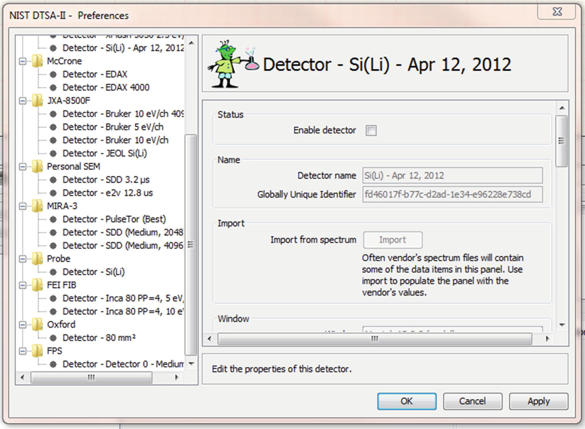
The preferences dialog showing a panel containing properties of a detector

To make optimal use of DTSA-II, you will need to create a detector model to describe each of your X-ray detectors. Each detector model reflects the performance of a specific detector in a specific instrument at a specific resolution/throughput setting. Each physical detector should be associated with at least one detector model. A single physical detector may have more than one detector model if the detector is regularly operated at different resolution / throughput settings.

Some of the information necessary to build the detector model is readily available from product literature or from a call to the vendor. Unfortunately, some pieces of information are less easy to discover. Some require access to very specialized samples or equipment, but fortunately, accepting the default values won’t overly affect utility of the simulated results. ◘ Table 17.1 identifies which values are critical and which are less critical.

Table 17.1

This table identifies parameters that have a critical influence on simulated spectra and those that have a less critical influence. You should be able to determine the correct value of the critical parameters from vendor literature or a call to the vendor. The vendor may be able to provide the less critical values too but if they can’t just accept the defaults

Critical	Less critical
Window type	Gold layer (accept the default)
Elevation angle	Aluminum layer (accept the default)
Optimal working distance	Nickel layer (accept the default)
Sample-to-detector distance (estimate)	Dead layer (accept the default)
Detector area	Zero strobe discriminator (easy to estimate)
Crystal thickness
Number of channels
Energy scale (nominal)
Zero offset (nominal)
Resolution at Mn Kα (approximate)
Azimuthal angle

Detector models are created in the “Preferences” dialog which is accessed through the “File → Preferences” main menu item. The tree view on the left side of the dialog allows you to navigate through various preference pages. By default, a root node labeled “Instruments and Detectors” is created with a branch called “Probe” and a leaf node called “Si(Li).” The branch “Probe” reflects a very basic traditional SEM/microprobe. The leaf “Si(Li)” reflects a typical lithium-drifted silicon detector with a ultra-thin window and a resolution of 132 eV at Mn Kα. You can examine the definition of this detector to determine which pieces of information are necessary to fully describe a detector.

Some pieces of information are specific to your instrument and the way the detector is mounted in the instrument. Window-type, detector area, crystal thickness, resolution, gold layer thickness, aluminum layer thickness, nickel layer thickness, and dead layer thickness are model specific properties of the detector. Elevation angle, optimal working distance, sample-to-detector distance, and azimuthal angle are determined by how the detector is mounted in your instrument. The energy scale, zero offset, and the resolution are dependent upon hardware settings that are usually configured within the vendor’s acquisition software. The oldest systems may have physical hardware switches.

Window Type (◘ Fig. 17.2)

Fig. 17.2

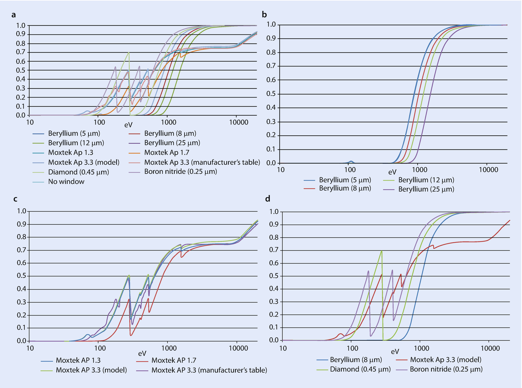
a–d: Window transmission efficiency as a function of photon energy

As is discussed elsewhere, most detectors are protected from contamination by an X-ray transparent window. Older windows were made of ultrathin beryllium foils or occasionally boron-nitride or diamond films. Almost all modern detectors use ultrathin polymer windows although the recently introduced silicon nitride (Si₃N₄) windows show great promise.

Each type of window has a different efficiency as a function of energy. The largest variation in efficiency is seen below 1 keV. Here the absorption edges in the elements making up the windows can lead to large jumps in efficiency over narrow energy ranges. Diamond represents an extreme example in which the absorption edge at 0.283 keV leads to a three order-of-magnitude change in efficiency.

Your vendor should be able to tell you the make and model of the window on your detector.

The Optimal Working Distance (◘ Figs. 17.3 and 17.4)

Fig. 17.3

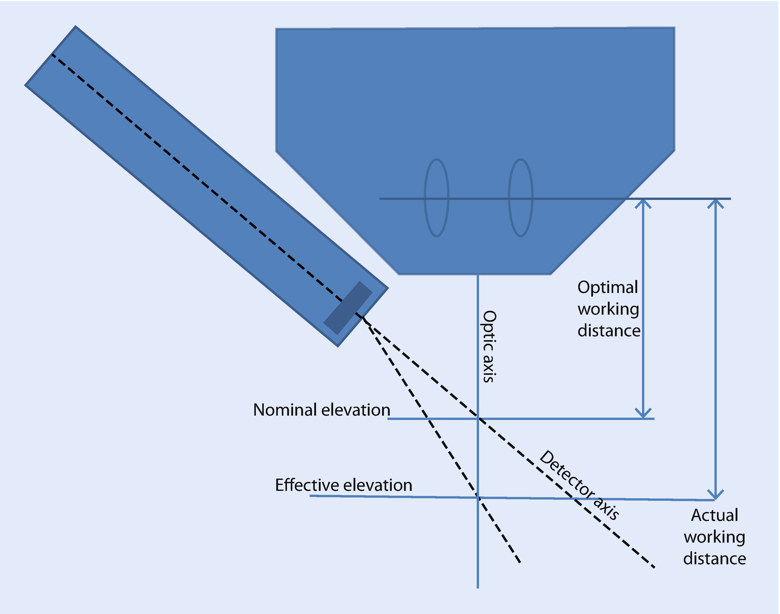
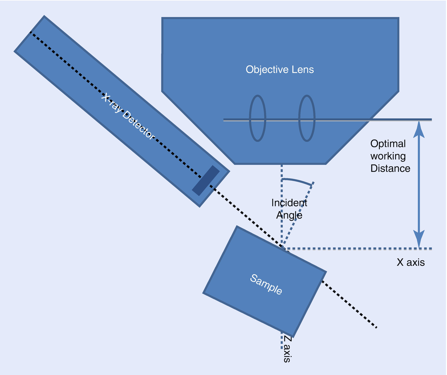
Definitions of geometric parameters

Fig. 17.4

Example of vendor-supplied schematics showing the optimal working distance (17 mm) and the sample-to-detector distance (34 mm) for a microscope with multiple detectors (Source: TESCAN)

The position and orientation of your EDS detector is optimized for a certain sample position. Typically, the optimal sample position is located on the electron-beam axis at an optimal working distance. At this distance, the effective elevation angle equals the nominal elevation angle. Sometimes, the optimal working distance will be specified in the drawings the EDS vendor used to design the detector mounting hardware (◘ Fig. 17.4). Other times, it is necessary to estimate the optimal working distance finding the sample position that produces the largest X-ray flux. The optimal working distance is measured on the same scale as the focal distance since the working distance value recorded in spectrum files is typically this value.

The difference between the effective elevation defined by the actual working distance and the nominal elevation as defined by the intersection of the detector axis and the optic axis. The effective elevation angle can be calculated from the actual working distance given the optimal working distance, the nominal elevation angle, and the nominal sample-to-detector distance.

Elevation Angle

The elevation angle is defined as the angle between the detector axis and the plane perpendicular to the optic axis. The elevation angle is a fixed property of the detector as it is mounted in an instrument. The elevation angle is closely related to the take-off angle. For a sample whose top surface is perpendicular to the optic axis, the take-off angle at the optimal working distance equals the elevation angle.

Elevation angles typically range between 30° and 50° with between 35° and 40° being the most common. The correct detector elevation is important for accurate quantification as the matrix correction has a strong dependence on this parameter.

Sample-to-Detector Distance

The sample-to-detector distance is the distance from front face of the detector crystal to the intersection of the optic and detector axes. The sample-to-detector distance helps to define the solid angle of acceptance for the detector. The sample-to-detector distance can often be extracted from the drawings used to design the detector mounting hardware (See ◘ Fig. 17.3).

Alternatively, you can estimate the distance and adjust the value by comparing the total integrated counts in a simulated spectrum with the total integrated counts in an equivalent measured spectrum. The simulated counts will decrease as the square in the increase of the sample-to-detector distance.

Detector Area

The detector area is the nominal surface area of the detector crystal visible (unobstructed) from the perspective of the optimal analysis point. The detector area is one of the values that detector vendors explicitly specify when describing a detector. Typical values of detector area are 5, 10, 30, 50, or 80 mm². The detector area does not account for area obstructed by grid bars on the window but does account for area obstructed by a collimator or other permanent pieces of hardware.

Crystal Thickness

The detection efficiency for hard (higher-energy) X-rays depends upon the thickness of the active detector crystal area. Si(Li) detectors tend to have much thicker crystals and thus measure X-rays with energies above 10 keV more efficiently. Silicon drift detectors (SDD) tend to be about an order of magnitude thinner and become increasingly transparent to X-rays above about 10 keV. DTSA-II defaults to a thickness of 5 mm for Si(Li) detectors and 0.45 mm for SDD. These values will work adequately for most purposes if a vendor specified value is unavailable.

Number of Channels, Energy Scale, and Zero Offset

A detector’s energy calibration is described by three quantities—the number of bins or channels, the width of each bin (energy scale), and the offset of the zero-th bin (zero offset). The number of bins is often a power-of-two, most often 2,048 but sometimes 1,024 or 4,096. This number represents the number of individual, adjacent energy bins in the spectrum. The width of each bin is assumed to be a nice constant—typically 10 eV, 5 eV, 2.5, or occasionally 20 eV. The detector electronics are then adjusted (in older systems through physical potentiometers or in modern systems through digital calibration) to produce this width.

The zero offset allows the vendor to offset (‘shift’) the energy scale for the entire spectrum by a fixed energy or to compensate for a slight offset in the electronics. Some vendors don’t make use of ability and the zero offset is fixed at zero. Other vendors use a negative zero offset to measure the full width of an artificial peak they intentionally insert into the data stream at 0 eV called the zero-strobe peak. The zero-strobe peak is often used to automatically correct for electronic drift. Often, DTSA-II can read these values from a vendor’s spectrum file using the “Import from spectrum” tool.

You don’t need to enter the exact energy scale and zero offset when you create the detector as the calibration tool can be used to refine these values.

Resolution at Mn Kα (Approximate)

The resolution is a measure of the performance of an EDS detector. Since the resolution depends upon X-ray energy in a predictable manner, the resolution is by long established standard reported as the “full width half maximum” (FWHM) of the Mn Kα peak (5.899 keV).

The full width at half-maximum is defined as the width of a peak as measured half way from the base to the peak. This is illustrated in the ◘ Fig. 17.5. The full height is measured from the level of the continuum background to the top of the peak. A line is drawn across the peak at half the full height. To account for the finite bin width, a line is drawn on each side of the peak from the center of the bin above the line to the center of the bin below the line. The intersection of this diagonal line is assumed to be the true peak edge position. The width is then measured from these intersection points and calibrated relative to the energy scale.

Fig. 17.5

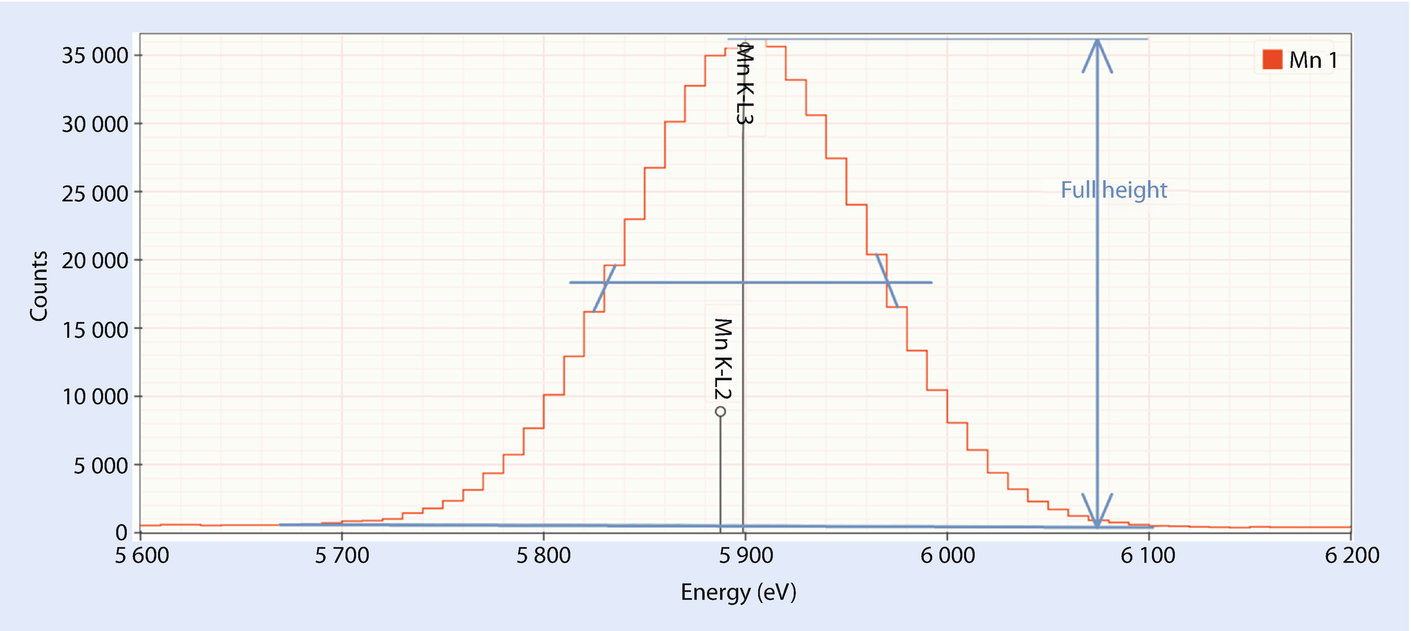
Estimating the full width at half-maximum peak width. This peak is approximately 139 eV FWHM which you can confirm with a ruler

The graphical method for estimating the FWHM is not as accurate as numerical fitting of Gaussian line shapes. The calibration tool uses the numerical method and is the preferred method (◘ Fig. 17.6).

Fig. 17.6

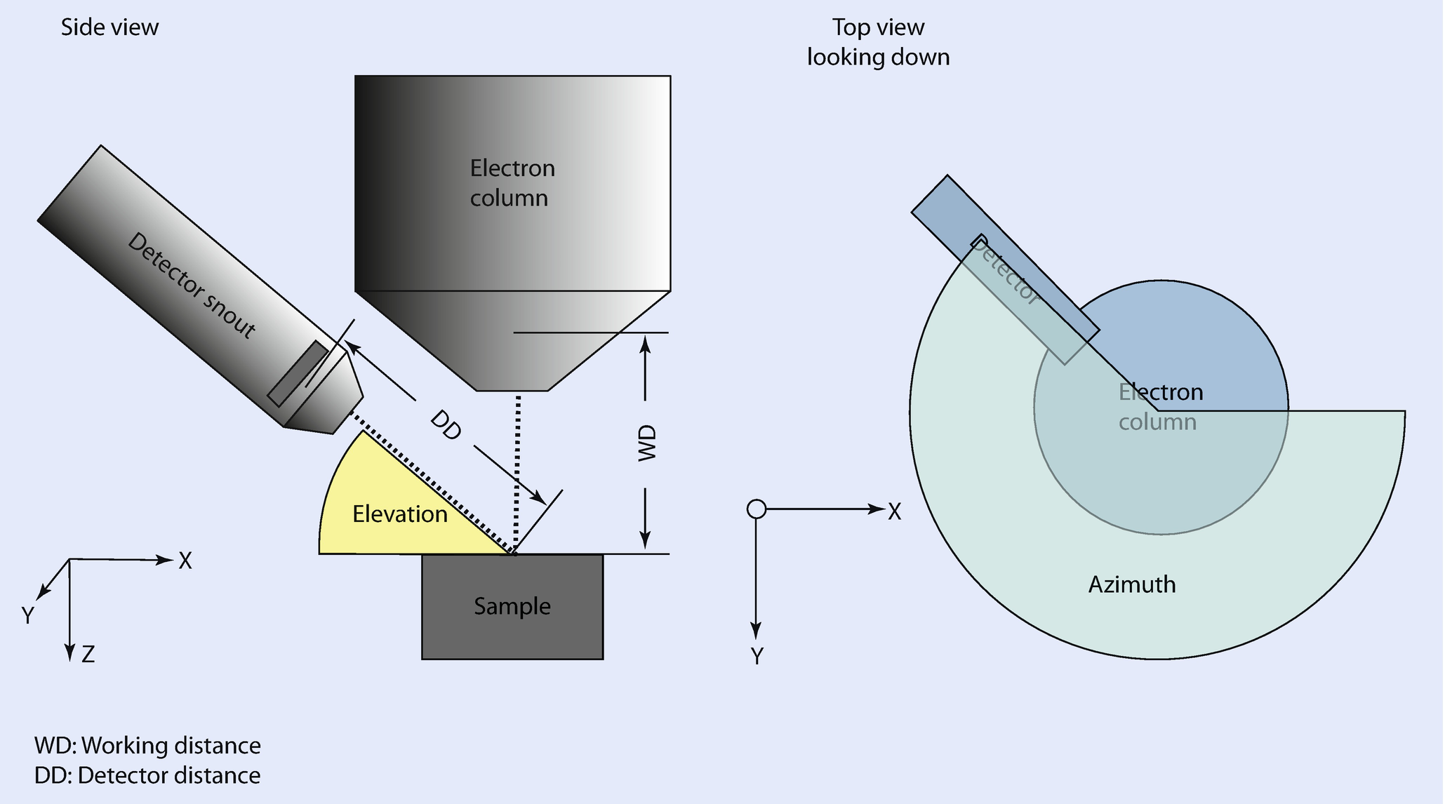
Definitions of elevation angle and azimuthal angle

Azimuthal Angle

The azimuthal angle describes the angular position of the detector rotated around the optic axis. The azimuthal angle is particularly important when modeling samples that are tilted or have complex morphology.

Gold Layer, Aluminum Layer, Nickel Layer

Detector crystals typically have conductive layers on their front face to ensure conductivity. These layers can be constructed by depositing various different metals on the surface. The absorption profiles of these layers will decrease the efficiency of the detector. The layer thicknesses are particularly relevant for simulation; however, other uncertainties usually exceed the effect of the conductive layer.

Dead Layer

The dead layer is an inactive or partially active layer of silicon on the front face of the detector. The dead layer will absorb some X-rays (particularly low energy X-rays) and produce few to no electron–hole pairs. The result is a fraction of X-rays which produce no signal or a smaller signal than their energy would suggest. The result is twofold: The first effect is a diminishment of the number of low energy X-rays detected. The second effect is a low energy tail, called incomplete charge collection, on low energy X-ray peaks.

The dead layer in modern detectors is very thin and typically produces very little incomplete charge collection. Older Si(Li) detectors had thicker layers and worse incomplete charge collection.

Zero Strobe Discriminator (◘ Figs. 17.7 and 17.8)

Fig. 17.7

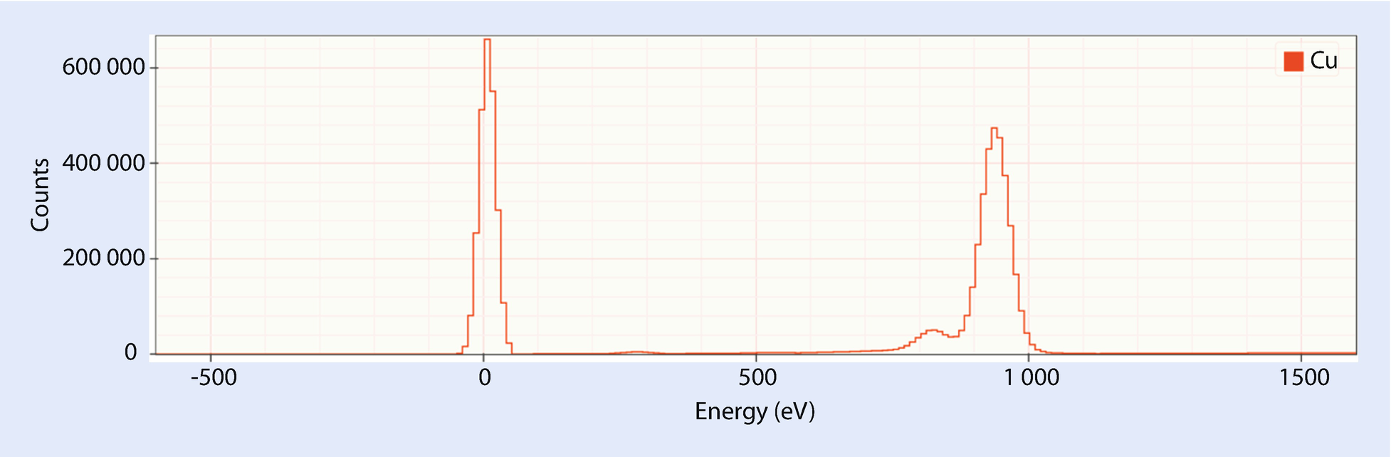
A raw Cu spectrum showing the zero strobe peak centered at 0 eV and the Cu L peaks centered near 940 eV

Fig. 17.8

The blue line shows an appropriate placement of the zero strobe discriminator between the high energy edge of the zero strobe and the start of the real X-ray data

The zero strobe discriminator is an energy below which all spectrum counts will be set to zero before many spectrum processing operations are performed.

The zero strobe is an artificial peak inserted by the detector electronics at 0 eV. The zero strobe is used to automatically determine the noise performance of the detector and to automatically adjust the offset of the detector to compensate for shifts in calibration. The zero strobe does not interfere with real X-ray events because it is located below the energies at which the detector is sensitive.

Some vendors automatically strip out the zero strobe out before presenting the spectrum. Others leave it in because it can provide useful information. When it does appear, it can negatively impact processing low energy peaks. To mitigate this problem, the zero strobe discriminator can be used to strip the zero strobe from the spectrum. The zero strobe discriminator should be set to an energy just above the high energy tail of the zero strobe.

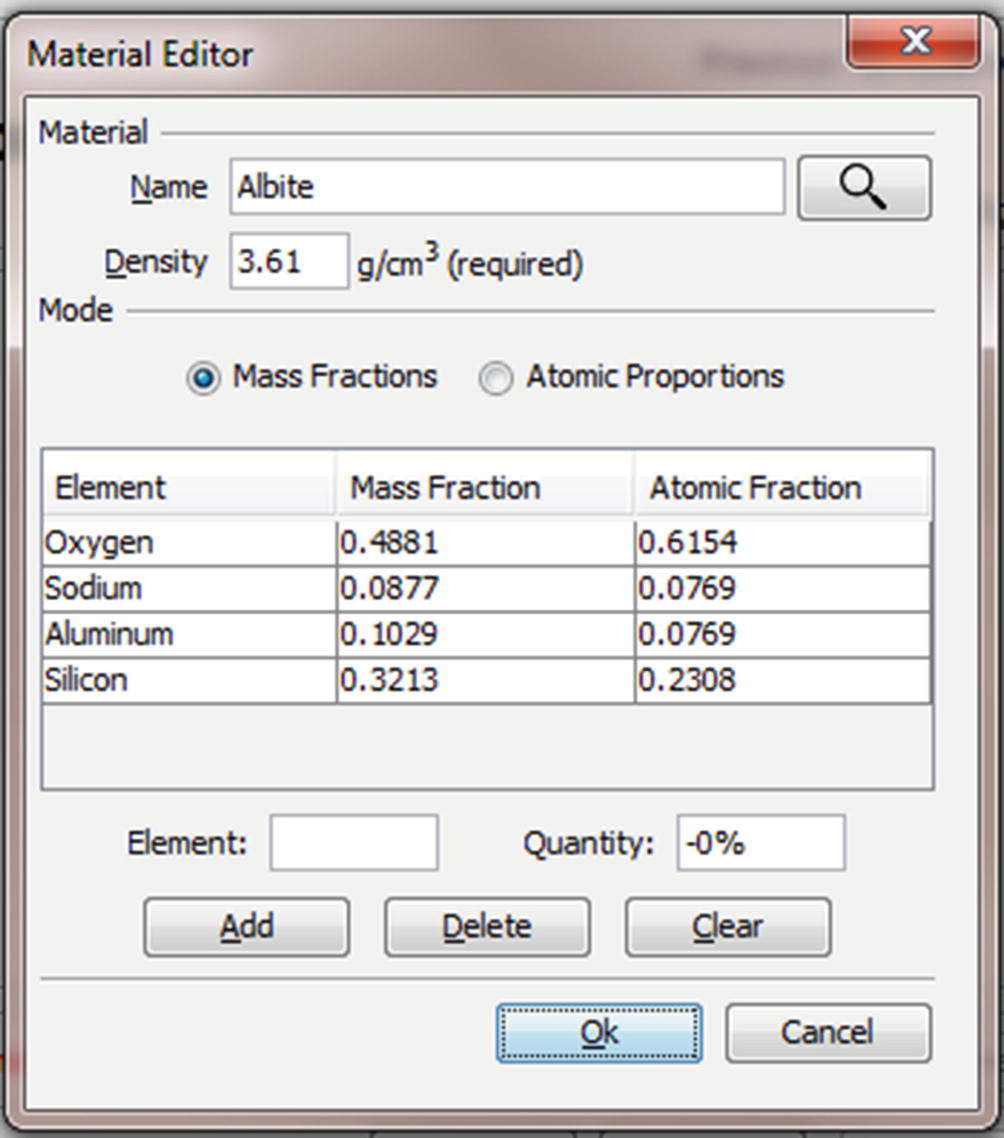
Material Editor Dialog (◘ Figs. 17.9, 17.10, 17.11, 17.12, 17.13, and 17.14)

Fig. 17.9

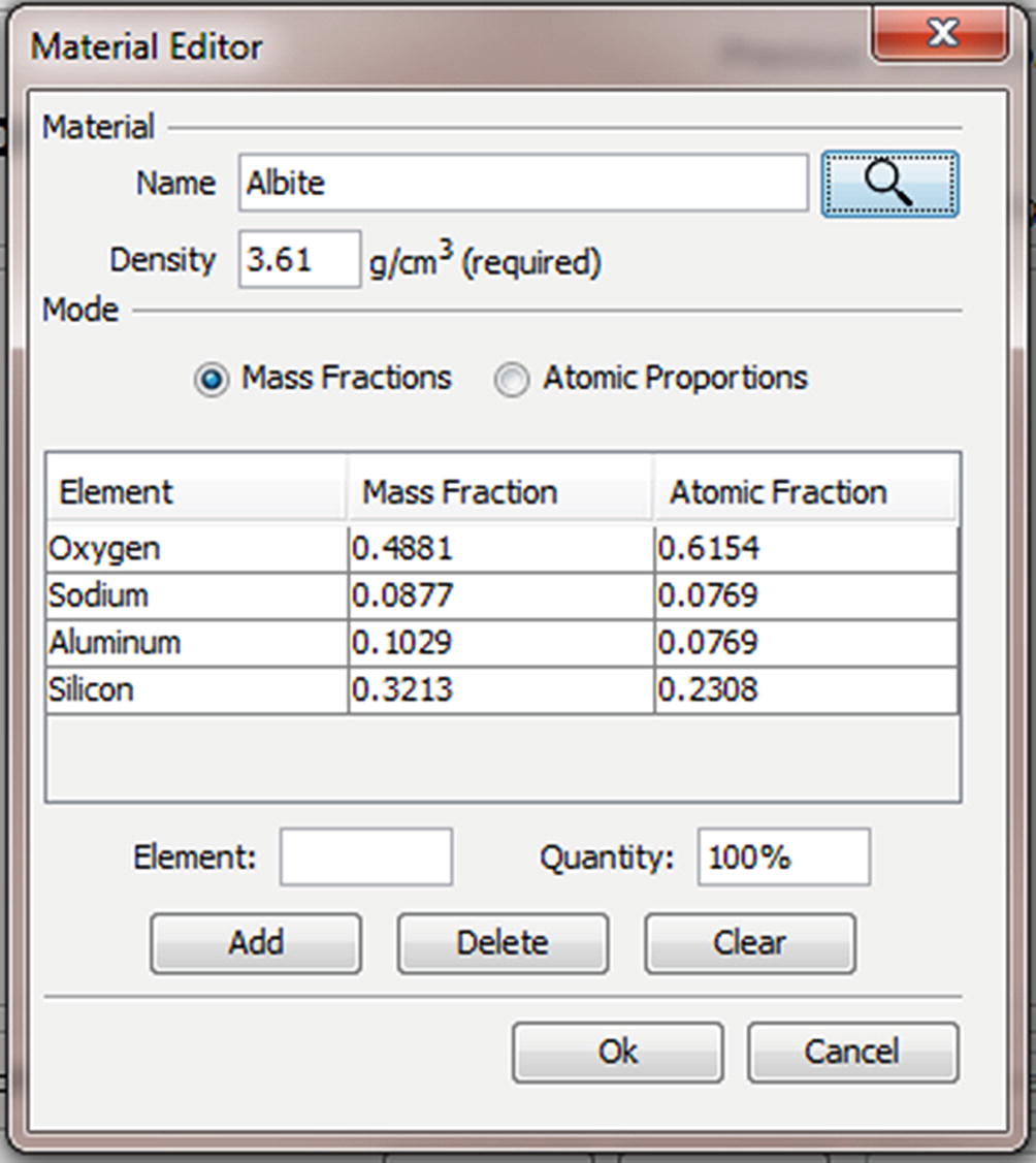
The material editor dialog. Materials are defined by a name (“Albite”), a density (“3.61 g/cm³”), and a mapping between elements and quantities. Albite is defined as NaAlSi₃O₈ which is equivalent to the mass fractions and atomic fractions displayed in the table

Fig. 17.10

The relative amount of each element in mass fractions may be entered manually using the “Element” and “Quantity” edit boxes and the “Add” button. Note that the mode radio button is set to “Mass Fractions” and that the quantity is entered in percent but displayed in mass fractions, so “10.29” corresponds to a mass fraction of “0.1029”. The element may be specified by the common abbreviation (“Al”), the full name (“aluminum”) or the atomic number (“13”)

Fig. 17.11

The relative amount of each element in atomic fractions may be entered manually using the “Element” and “Quantity” edit boxes and the “Add” button. Note that the mode radio button is set to “Atomic Proportions” and that the quantity is entered as a number of atoms in a unit cell. The element may be specified by the common abbreviation (“Si”), the full name (“silicon”) or the atomic number (“14”)

Fig. 17.12

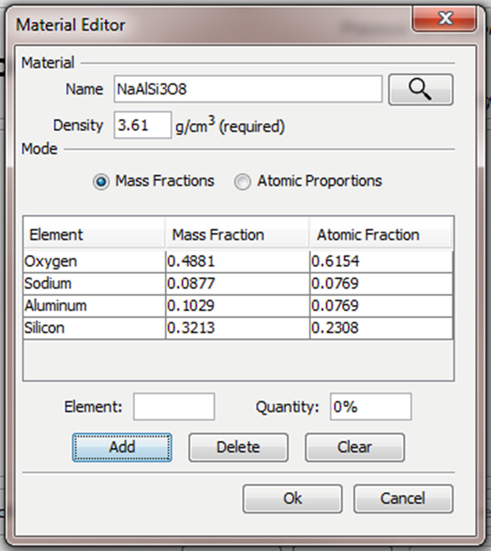
It is possible to enter the chemical formula directly into the “Name” edit box. When the search button is pressed the chemical formula will be parsed and the appropriate mass and atomic fractions entered into the table. Capitalization of the element abbreviations is important as “CO” is very different from “Co”—one is a gas and the other a metal. More complex formulas like fluorapatite (“Ca₅(PO₄)₃F”) can be entered using parenthesis to group terms. It is important that the formula is unambiguous. Once the formula has been parsed you may specify a new operator friendly name for the material like “Albite” of “Fluorapatite” in the “Name” edit box

Fig. 17.13

To assist the user, DTSA-II maintains a database of materials. Each time the user enters a new material or redefines an old material, the database is updated. The database is indexed by “Name”

Fig. 17.14

Albite (“NaAlSi₃O₈”) and anorthite (“CaAl₂Si₂O₈”) represent end members of the plagioclase solid solution series. To calculate a admixture of 50 % by mass albite and 50 % by mass anorthite, you can enter the formula “0.5*NaAlSi3O8 + 0.5*CaAl2Si2O8”. Other admixtures of stoichiometric compounds can be calculated in a similar manner. Remember to provide a user friendly name for the database

The material editor dialog is used to enter compositional and density information throughout DTSA-II. This dialog allows you to enter compositional information either as mass fractions or atomic fractions. It also provides shortcut mechanisms for looking up definitions in a database or entering compositions using the chemical formula.

• Method 1: Mass fractions (see ◘ Fig. 17.10)

• Method 2: Atomic fractions (see ◘ Fig. 17.11)

• Method 3: Chemical formula (see ◘ Fig. 17.12)

• Method 4: Database lookup (see ◘ Fig. 17.13)

• Method 5: Advanced chemical formulas (see ◘ Fig. 17.16)

So if your database contains a definition for “Albite” and you press the search button , the table will be filled with the mass and atomic fractions and the density as recorded in the database for “Albite.” The database is updated each time you select the “Ok” button. Over time, it is possible to fill the database with every material that you commonly see in your laboratory. The name “unknown” is special and is never saved to the database.

17.2 Simulation in DTSA-II

17.2.1 Introduction

Simulation, particularly Monte Carlo simulation, is a powerful tool for understanding the measurement process. Without the ability to visualize how electrons and X-rays interact with the sample, it can be very hard to predict the significance of a measurement. Does the incident beam remain within the sample? Where are the measured X-rays coming from? Can I choose better instrumental conditions for the measurements? Without simulation, these insight can only be gained with years of experience or based on simple rules of thumb.

Too often we are asked to analyze non-ideal samples. Monte Carlo simulation is one of the few mechanisms we have to ground-truth these measurements. Consider the humble particle. When is it acceptable to consider a particle to be essentially bulk and what are the approximate errors associated with this assumption?

17.2.2 Monte Carlo Simulation

Monte Carlo models are particularly useful because they permit the simulation of arbitrarily complex sample geometries. NIST DTSA-II provides a handful of different common geometries through the graphical user interface. More complex geometries can be simulated using the scripting interface.

Monte Carlo modeling is based on simulating the trajectories of thousands of electrons and X-rays. The simulated electrons are given an initial energy and trajectory which models the initial energy and trajectory of electrons from an SEM gun. The simulated electrons scatter and lose energy as their trajectories take them through the sample. Occasionally, an electron may ionize an atom and generate a characteristic X-ray. Occasionally, an electron may decelerate and generate a bremsstrahlung photon. The X-rays can be tracked from the point of generation to a simulated detector. A simulated spectrum can be accumulated. If care is taken modeling the electron transport and the X-ray interactions, the simulated spectrum can mimic a measured spectrum. Other data such as emitted intensities, emission images, trajectory images and excitation volumes can be accumulated.

Multi-element materials are modeled as mass-fraction averaged mixtures of elements. Complex sample geometries can be constructed out of discrete sample shapes that include blocks, spheres, cylinders, regions bounded by planar surfaces, and sums and differences of the basic shapes. In this way, it is possible to model arbitrarily complex sample geometries.

17.2.3 Using the GUI To Perform a Simulation

The simplest way to simulate one of an array of common sample geometries in through the “simulation alien.” The “simulation alien” is a dialog that takes you step-by-step through the process of simulating an X-ray spectrum. The dialog requests information that defines the sample geometry, the instrument, and detector, the measurement conditions and the information to simulate. The results of the simulation include a spectrum, raw intensity data, electron trajectory images, X-ray emission images, and excitation volume information. The “simulation alien” is accessed through the “Tools” application menu (◘ Fig. 17.15).

Fig. 17.15

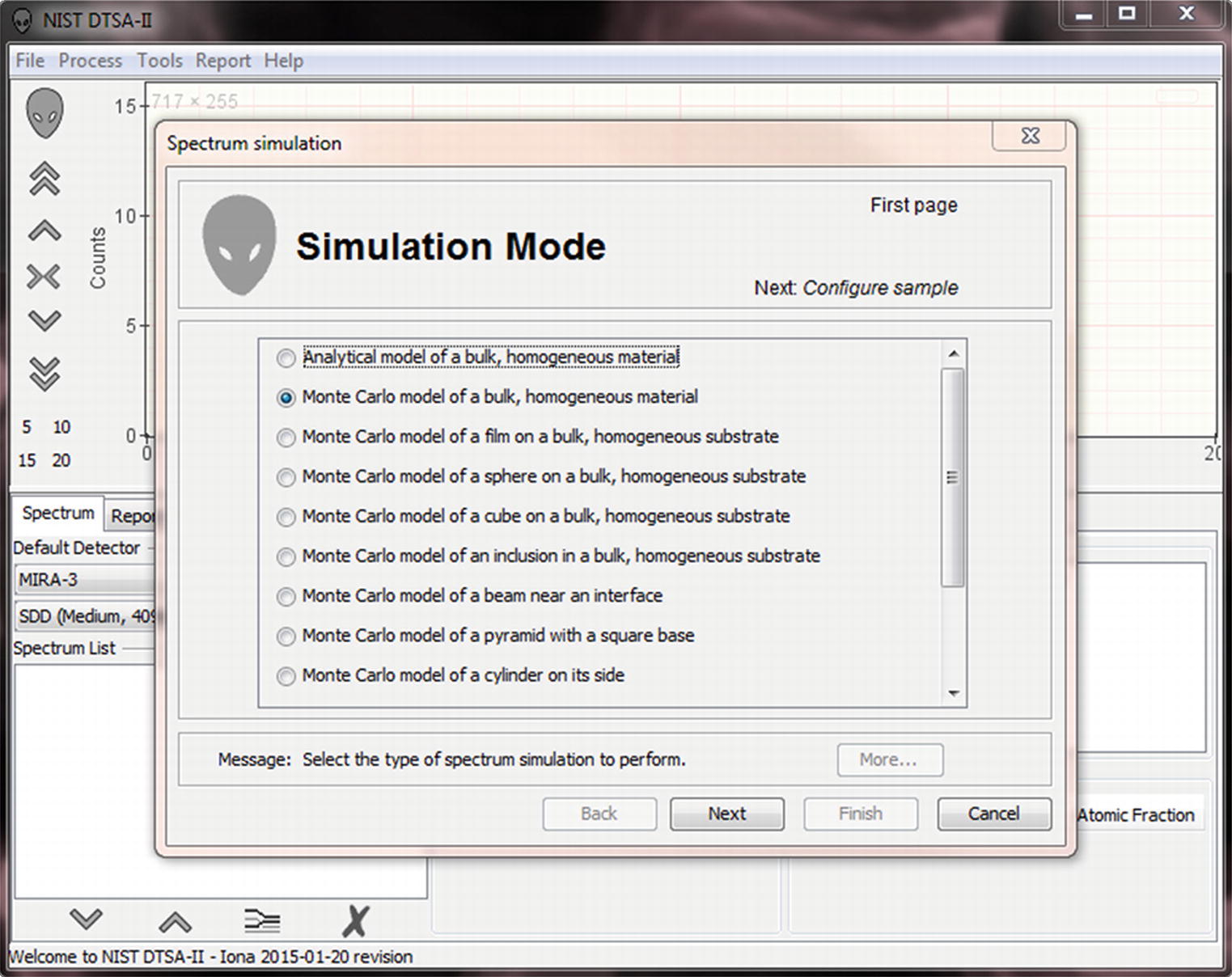
Simulation mode window in DTSA-II

Many different common sample geometries are available through the “simulation alien.”

• Analytical model of a bulk, homogeneous material.

  • A φ(ρz)-based analytical spectrum simulation model. This model simulates a spectrum in a fraction of a second but is only suited to bulk samples.

• Monte Carlo model of a bulk, homogeneous material.

  • The Monte Carlo equivalent of the φ(ρz)-based analytical spectrum simulation model (see ◘ Fig. 17.16).

• Monte Carlo model of a film on a bulk, homogeneous substrate.

  • A model of a user specified thickness film on a substrate (or, optionally, unsupported) (see ◘ Fig. 17.17).

• Monte Carlo model of a sphere on a bulk, homogeneous substrate (see ◘ Fig. 17.18).

  • A model of a user specified radius sphere on a substrate (or, optionally, unsupported).

• Monte Carlo model of a cube on a bulk, homogeneous substrate.

  • A model of a user specified size cube on a substrate (or, optionally, unsupported) (see ◘ Fig. 17.19).

• Monte Carlo model of an inclusion on a bulk, homogeneous substrate.

  • A model of a block inclusion of specified square cross section and specified thickness in a substrate (or, optionally, unsupported) (see ◘ Fig. 17.20).

• Monte Carlo model of a beam near an interface.

  • A model of two materials separated by a vertical interface nominally along the y-axis. The beam can be placed a distance from the interface in either material. Positive distances place the beam in the primary material and negative distances are in the secondary material (see ◘ Fig. 17.21).

• Monte Carlo model of a pyramid with a square base.

  • The user can specify the length of the base edge and the height of the pyramid (see ◘ Fig. 17.22).

• Monte Carlo model of a cylinder on its side

  • The user can specify the length and diameter of the cylinder (see ◘ Fig. 17.23).

• Monte Carlo model of a cylinder on its end

  • The user can specify the length and diameter of the cylinder (see ◘ Fig. 17.24).

• Monte Carlo model of a hemispherical cap

  • The user can specify the radius of the hemispherical cap (see ◘ Fig. 17.25).

• Monte Carlo model of a block

  • The user can specify the block base (square) and the height.

• Monte Carlo model of an equilateral prism

  • The user can specify the edge of the triangle and the length of the prism (◘ Figs. 17.16, 17.17, 17.18, 17.19, 17.20, 17.21, 17.22, 17.23, 17.24, 17.25, 17.26, 17.27, and 17.28).

    

    Fig. 17.16

    Bulk, homogeneous material

    

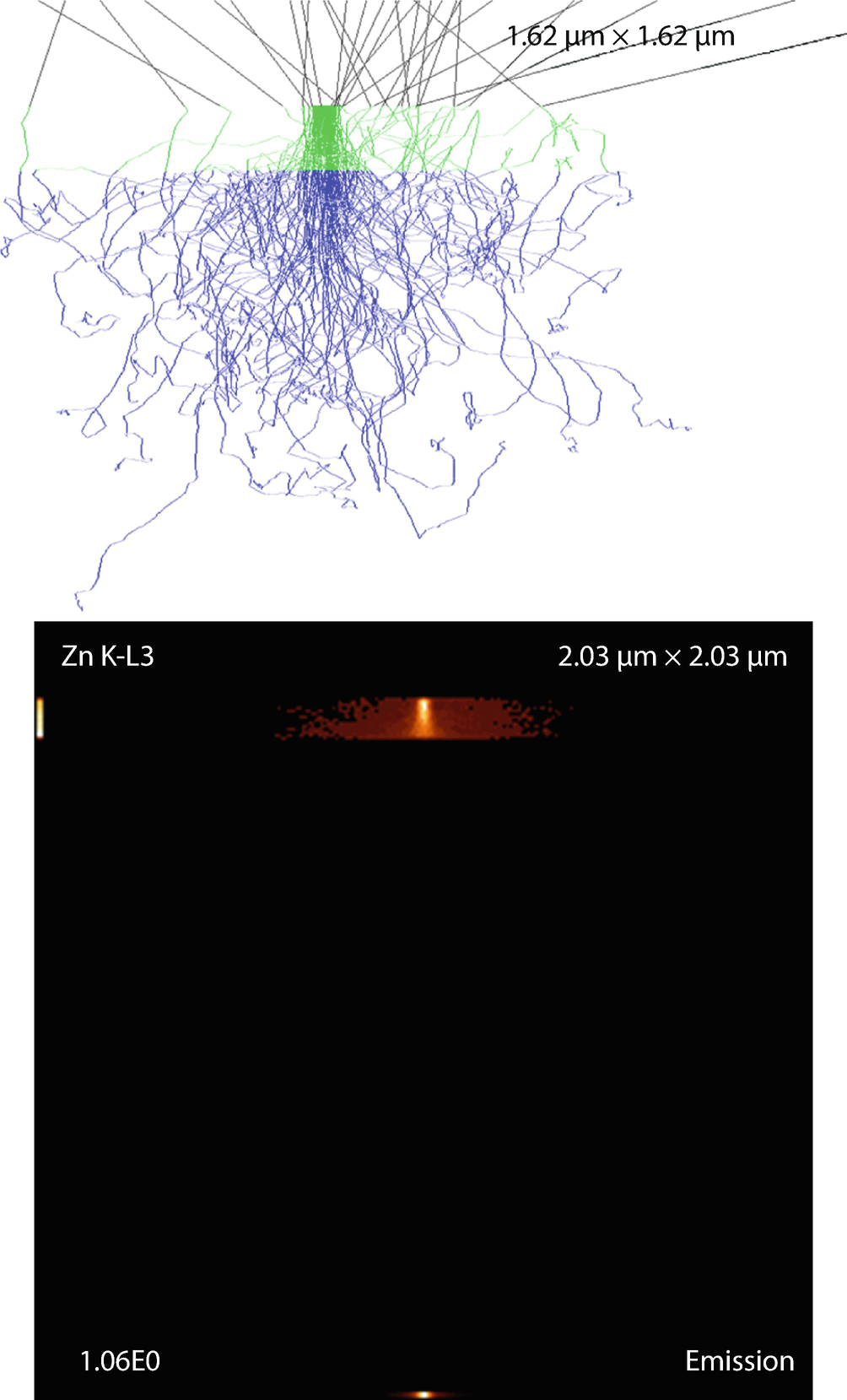    Fig. 17.17

    Thin film on substrate. Parameters: film thickness

    

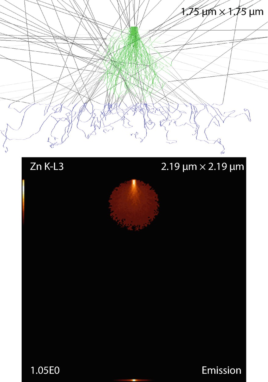    Fig. 17.18

    Spherical particle on a substrate. Parameters: Sphere’s radius

    

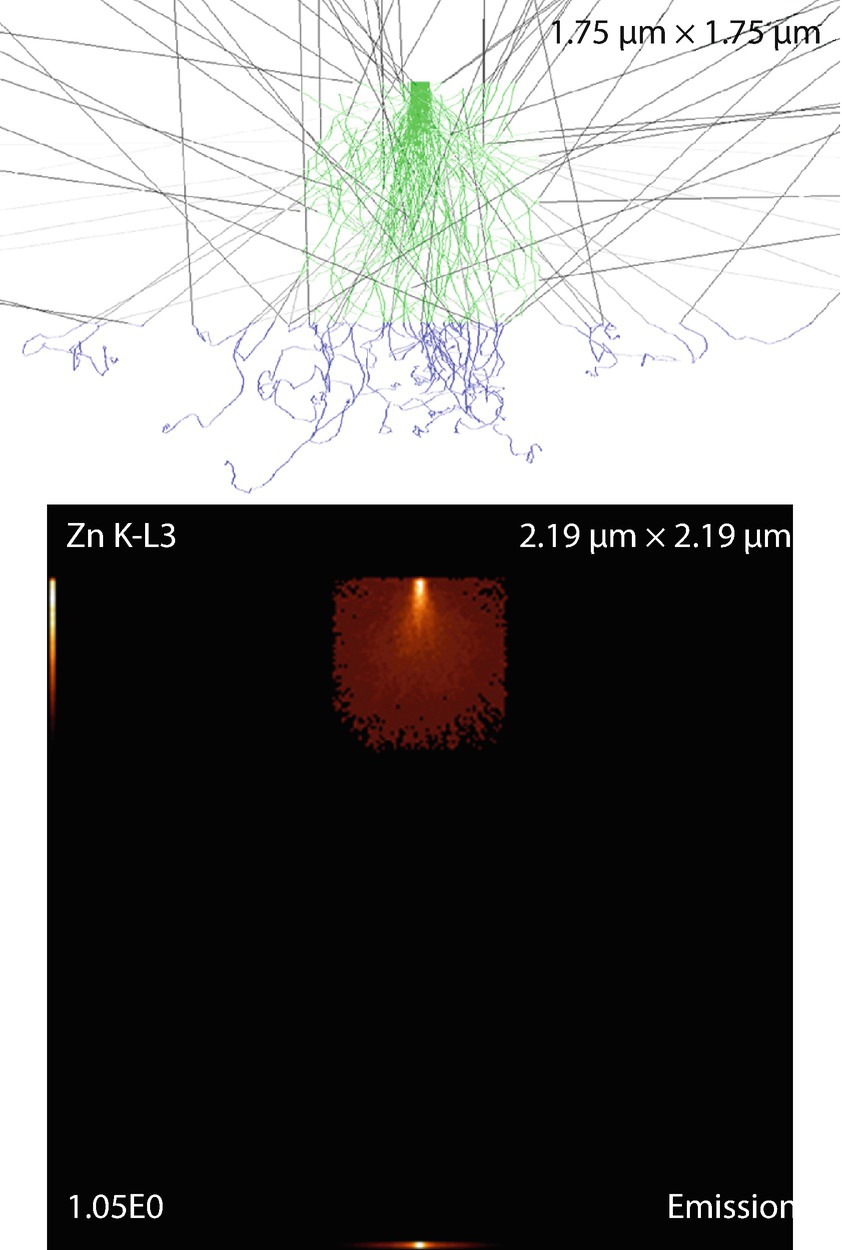    Fig. 17.19

    Cubic particle on a substrate. Parameters: Cube dimension

    

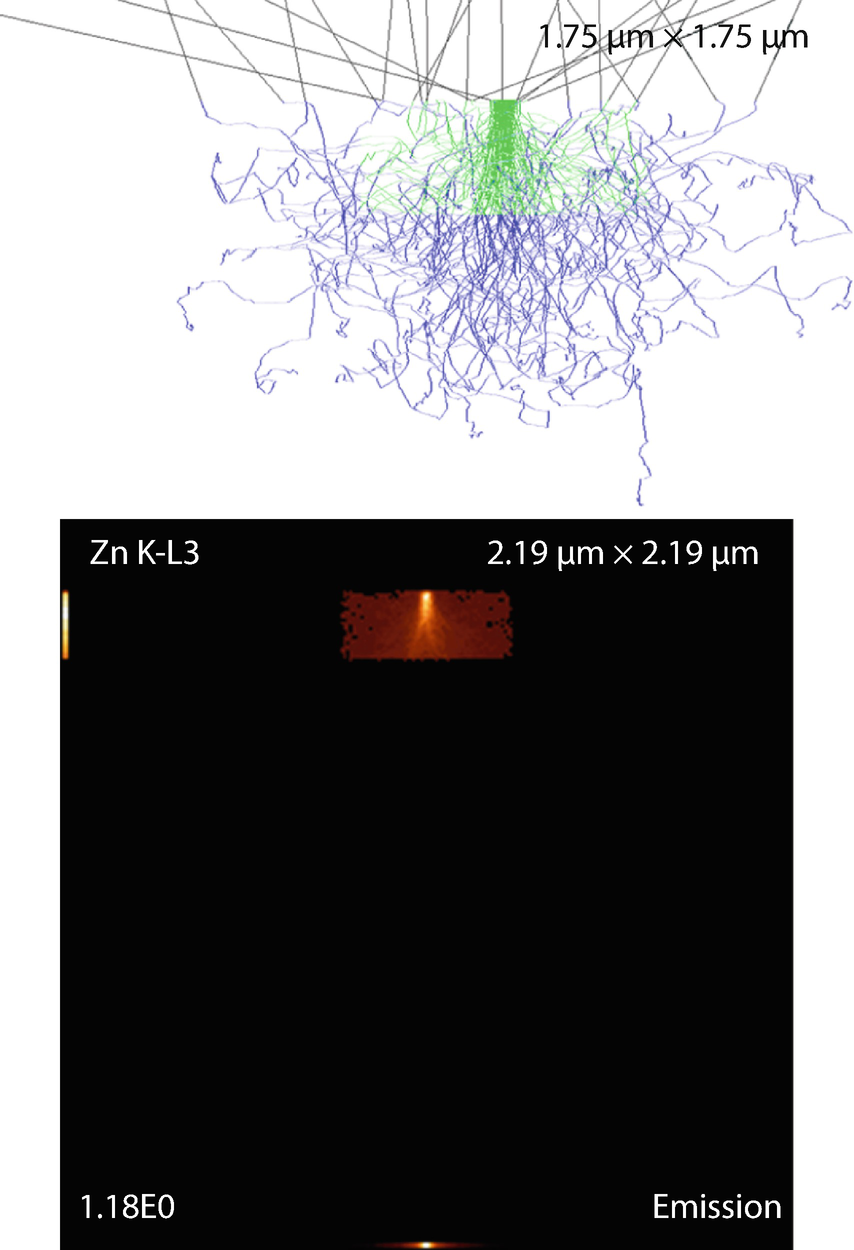    Fig. 17.20

    Block inclusion in substrate. Parameters: Thickness and edge length

    

    Fig. 17.21

    Interface between two materials. Parameters: Distance from interface

    

    Fig. 17.22

    Square pyramid on a substrate. Parameters: Height and base edge length

    

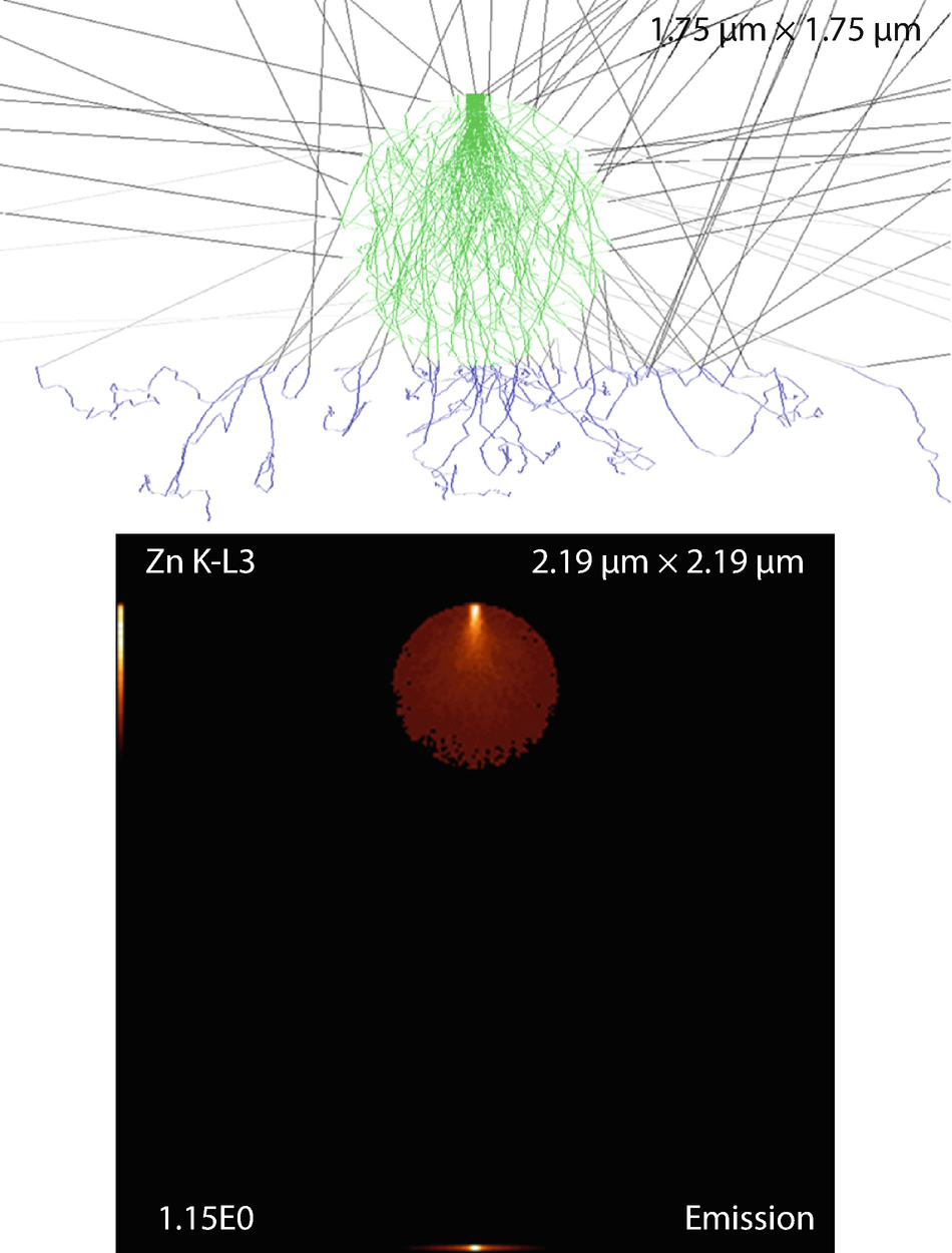    Fig. 17.23

    Cylinder (fiber) on substrate. Parameters: Fiber diameter and length

    

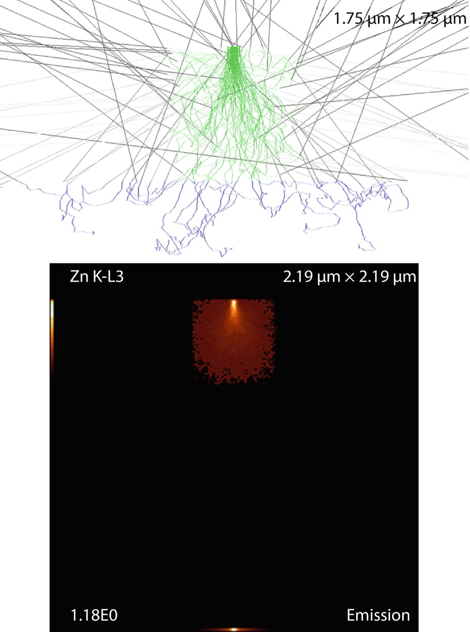    Fig. 17.24

    Cylinder (can) on end on substrate. Parameters: Height and fiber diameter

    

    Fig. 17.25

    Hemispherical cap on substrate. Parameters: Cap radius

    

    Fig. 17.26

    Rectangular block on substrate. Parameters: Block height and base edge length

    

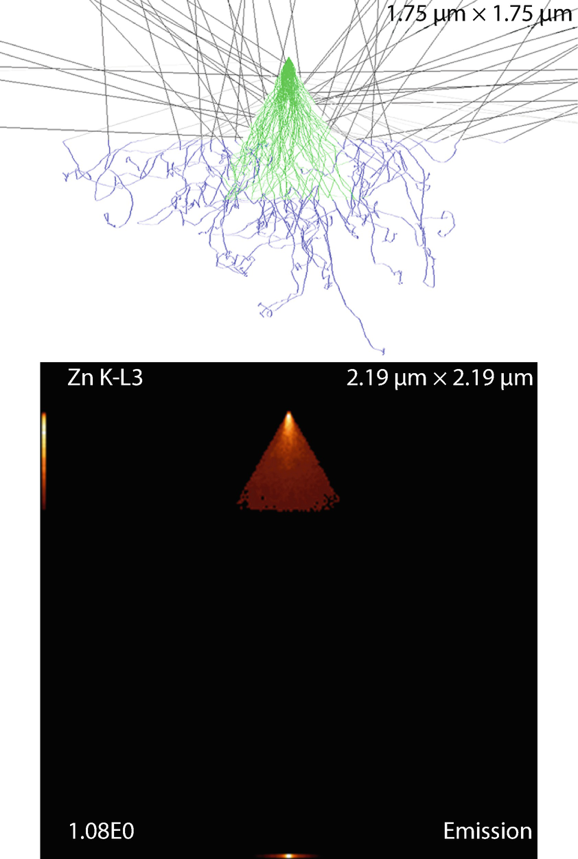    Fig. 17.27

    Triangular prism on substrate. Parameters: Triangle edge and prism lengths

    

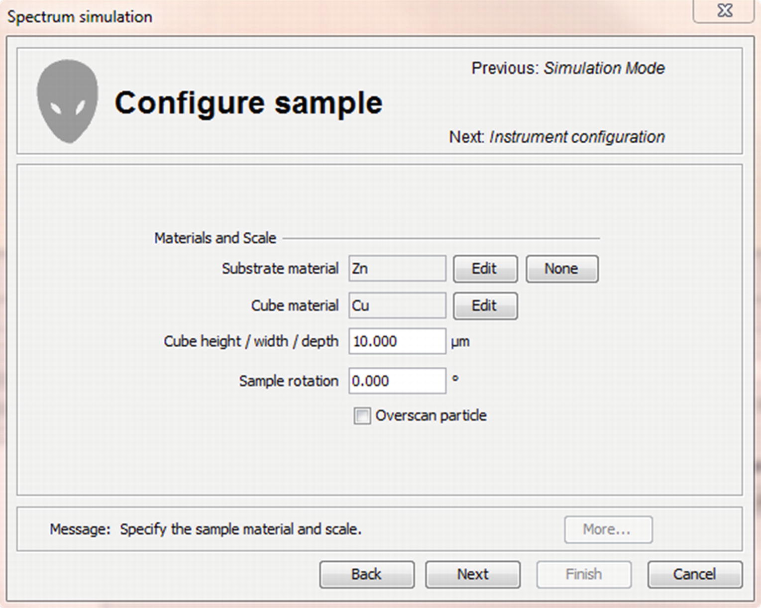    Fig. 17.28

    “Configure sample” menu

Each simulation mode takes different parameters to configure the sample geometry. This page is for the simulation of a cube which requires two materials (substrate and cube), the dimensions of the cube and the sample rotation.

The sample rotation parameter is available for all modes for which are not rotationally invariant. The best way to understand the sample rotation parameter is to imagine rotating the sample about the optic axis at the point on the sample at which the beam intersects (◘ Figs. 17.29, 17.30, and 17.31).

Fig. 17.29

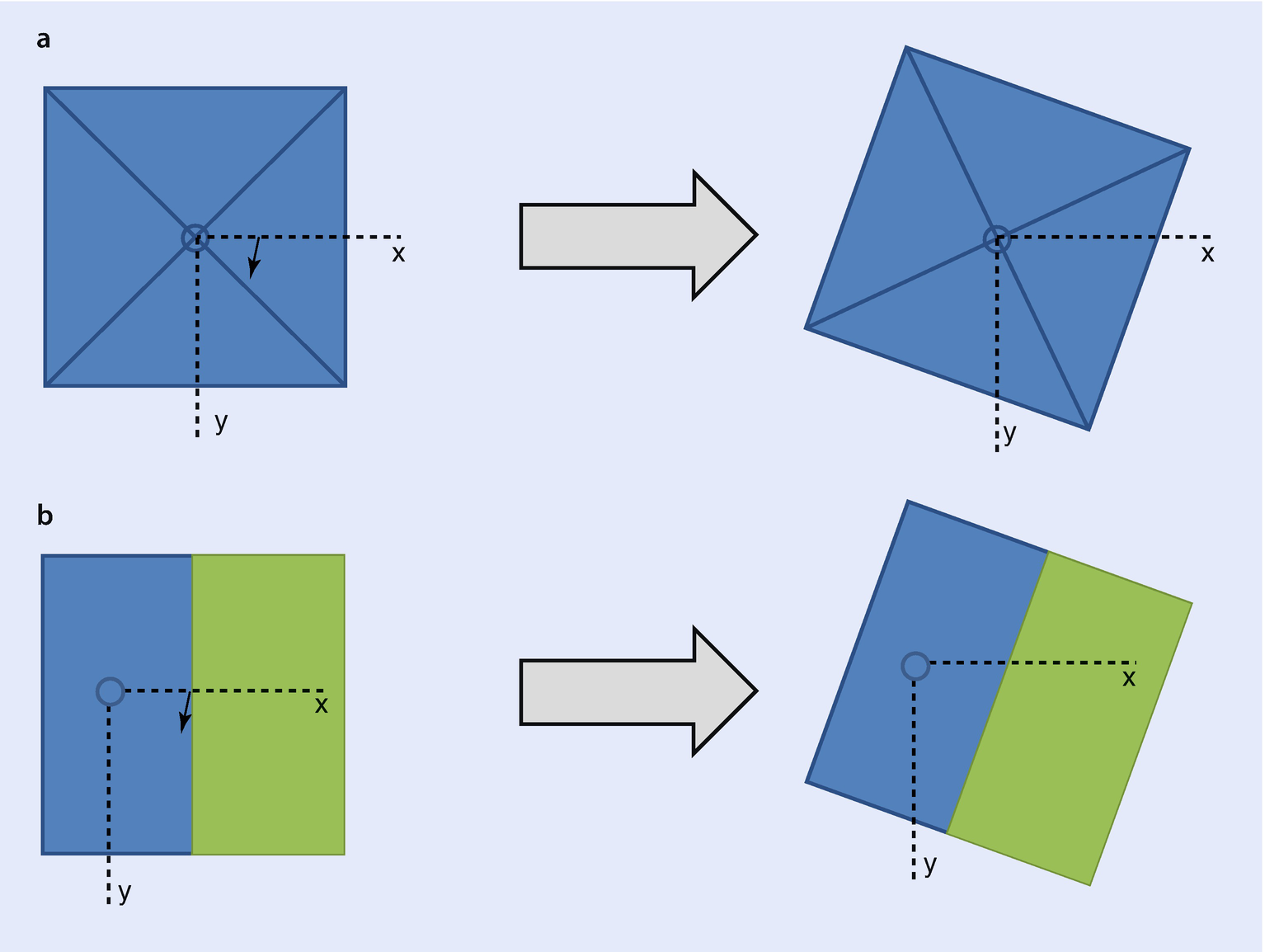
a Shows how a pyramid with square base model rotates and b shows how a beam near an interface model rotates. Both figures take the perspective of looking down along the optic axis at the sample. The shortest distance to the interface is maintained in ◘ figure b

Fig. 17.30

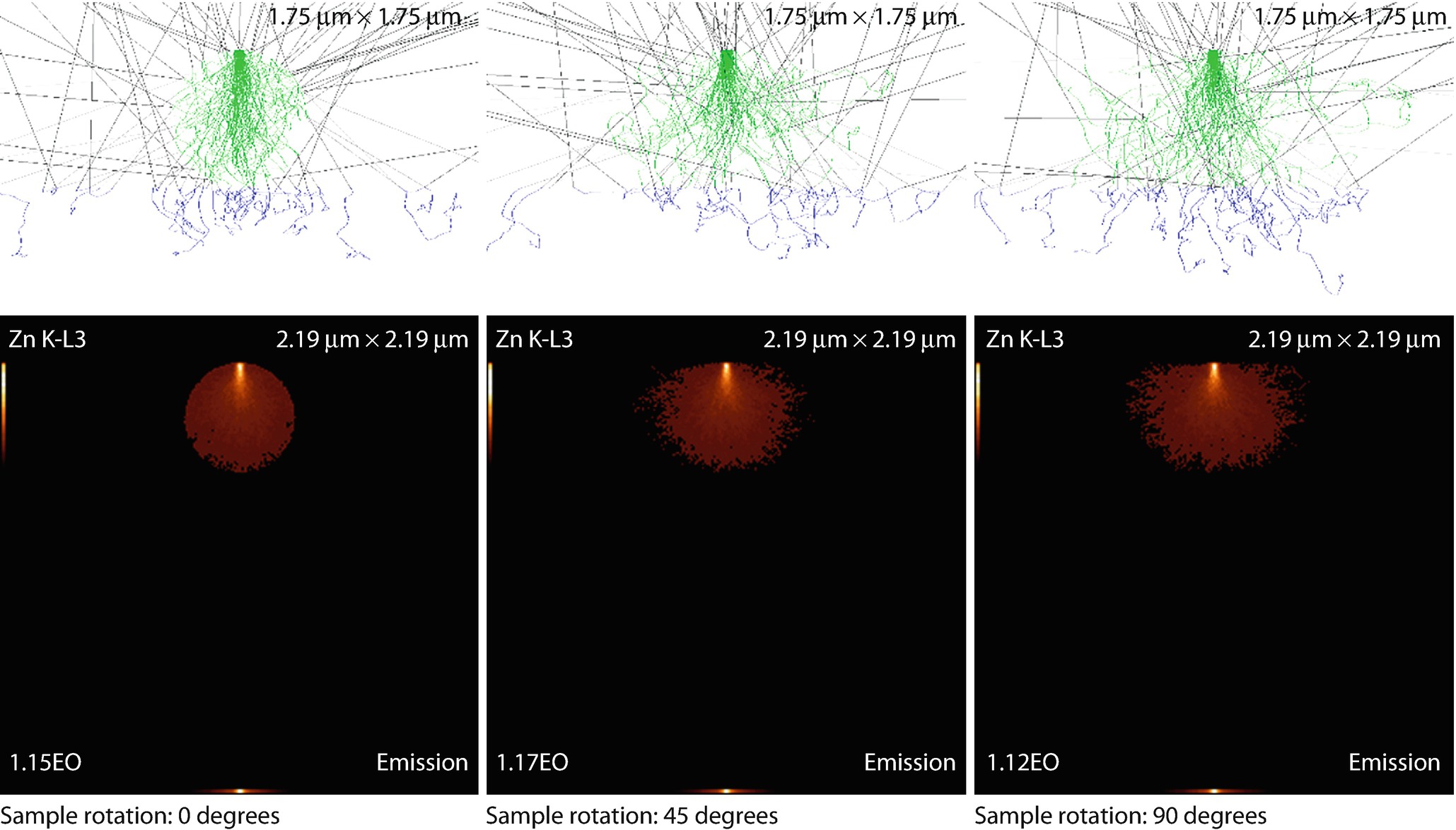
A fiber rotated through 0°, 45°, and 90°

Fig. 17.31

“Material editor” menu

All the models require you to specify at least one material. The material editor (described elsewhere) allows you to specify the material. Since the density is a critical parameter, you must specify it (◘ Fig. 17.32).

Fig. 17.32

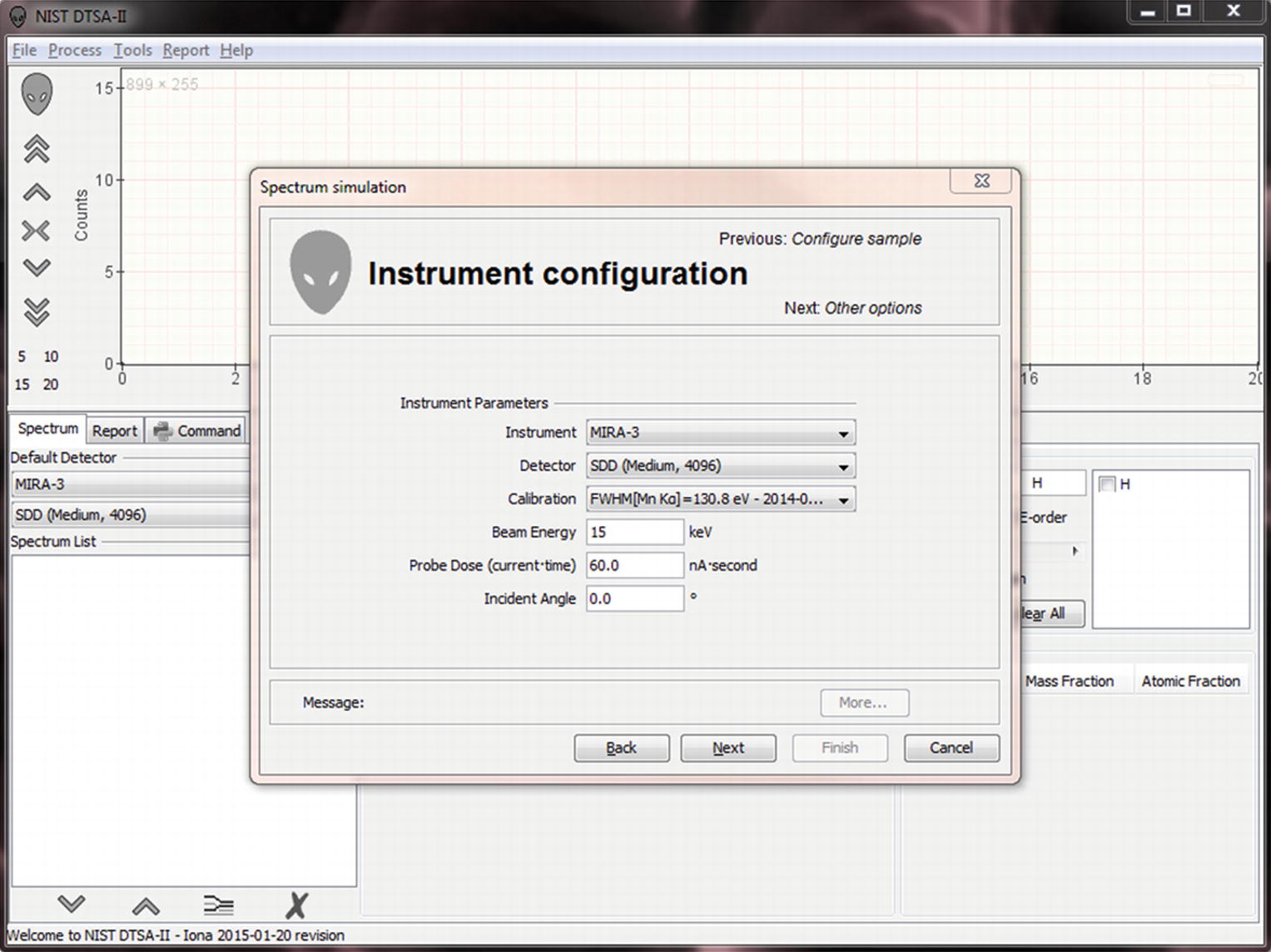
“Instrument configuration” menu

Simulations are designed to model the spectra you could collect on your instrument with your detector. By default, the simulation “instrument configuration” page assumes that you want to simulate the “default detector” as specified on the main “Spectrum” tab. However, you can specify a different instrument, detector and calibration if you desire.

You also need to specify an incident beam energy. This is the kinetic energy with which the electrons strike the sample and is specified in kilo-electronvolts (keV).

The probe dose determines the relative intensity in the spectrum. Probe dose is specified in nano-amp seconds (nA · s = nC). This quantity is a product of the probe current (nA) and the spectrum acquisition live-time (seconds.) Remember the probe current is a measure of the actual number of electrons striking the sample per unit time, so the probe dose is equivalent to a number of electrons striking the sample during the measurement. Doubling the dose doubles the number of electrons striking the sample and thus also doubles the average number of X-rays generated in the sample.

The incidence angle (nominally 0°) allows you to simulate a tilted sample (◘ Fig. 17.33).

Fig. 17.33

Definition of angles for a tilted specimen

The incident angle is defined relative to the optic axis. The pivot occurs at the surface of the sample, which is placed at the detector’s optimal working distance. A positive rotation is towards the X-axis (an azimuth of 0°) and a negative rotation towards the –X axis (an azimuth of 180°.) The detector displayed is at an azimuth of 180°. A negative incidence angle would tilt the sample toward the detector. Arbitrary tilts may be simulated by moving the detector around the azimuth (◘ Figs. 17.33, 17.34, 17.35, and 17.36).

Fig. 17.34

Tilting a bulk sample

Fig. 17.35

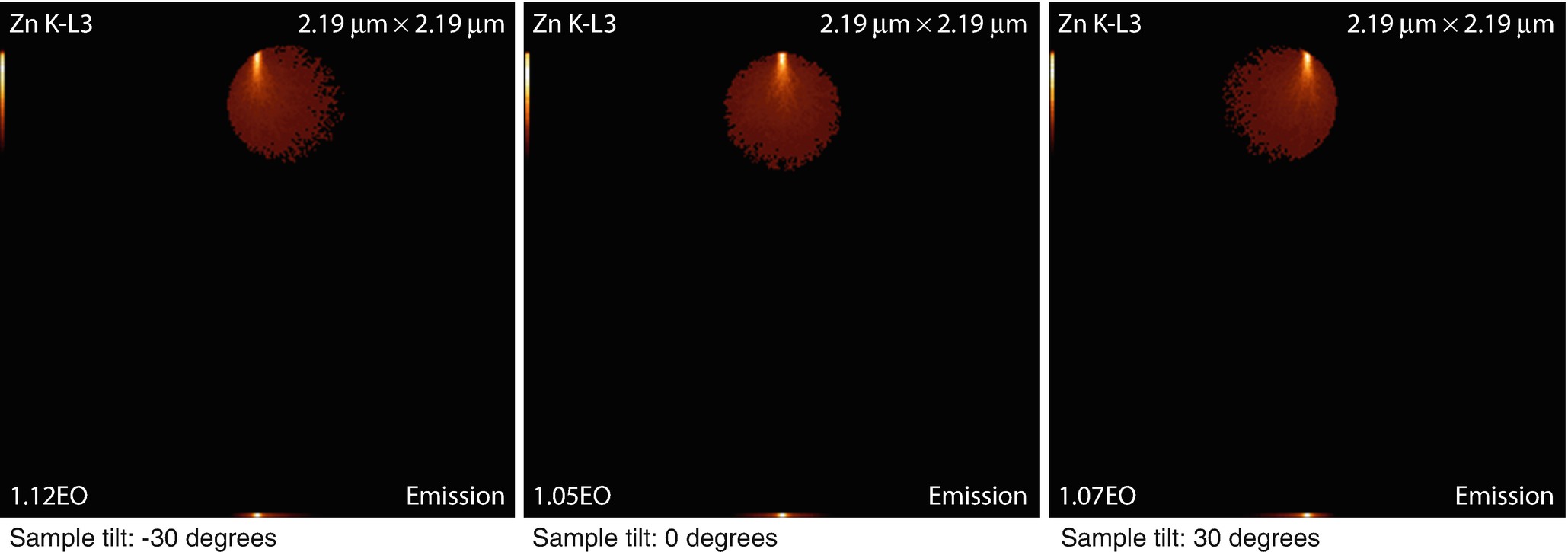
Tilting a spherical sample

Fig. 17.36

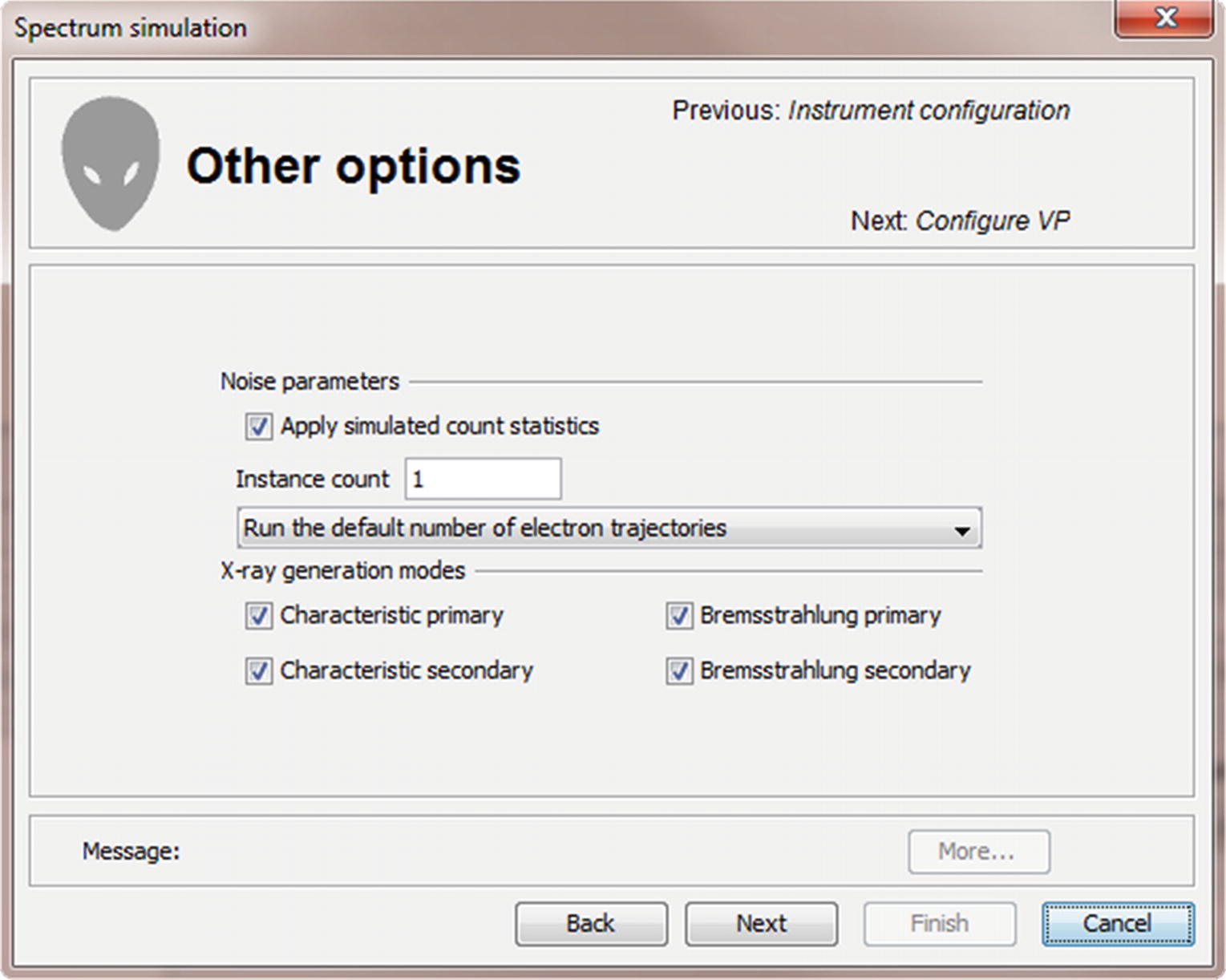
Menu for selecting number of trajectories, repetitions, and X-ray generation modes

The “other options” page allows you to specify whether the spectrum is simulated with or without variance due to count statistics. If you select to “apply simulated count statistics,” you may also select to output multiple spectra based on the simulated spectrum but differ by pseudorandom count statistics. You may also select to run additional simulated electron trajectories. The number of simulated electron trajectories determines the simulation to simulation variance in characteristic X-ray intensities. The default number of electron trajectories typically produces about 1 % variance. The variance decreases as the square-root of the number of simulated trajectories. You may also specify which X-ray generation modes to simulate including both characteristic and bremsstrahlung primary emission and secondary emission due to characteristic primary emission or bremsstrahlung primary emission (◘ Figs. 17.37, 17.38, and 17.39).

Fig. 17.37

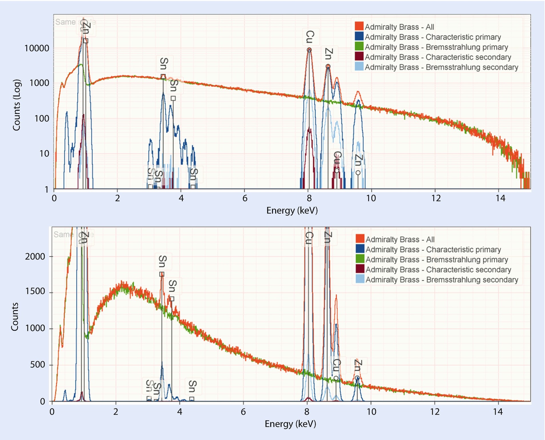
Simulated admiralty brass (69 % Cu, 30 % Zn, and 1 % Tin) for various different selections of generation modes

Fig. 17.38

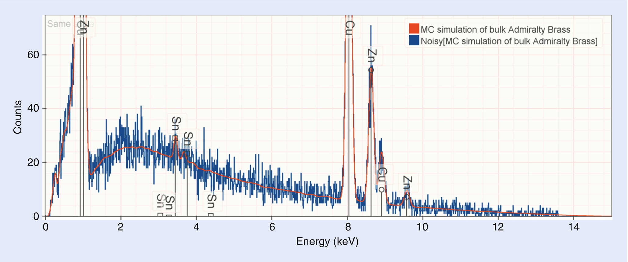
Simulated admiralty brass (69 % Cu, 30 % Zn, and 1 % Tin) with (blue) and without (red) simulated variation due to count statistics

Fig. 17.39

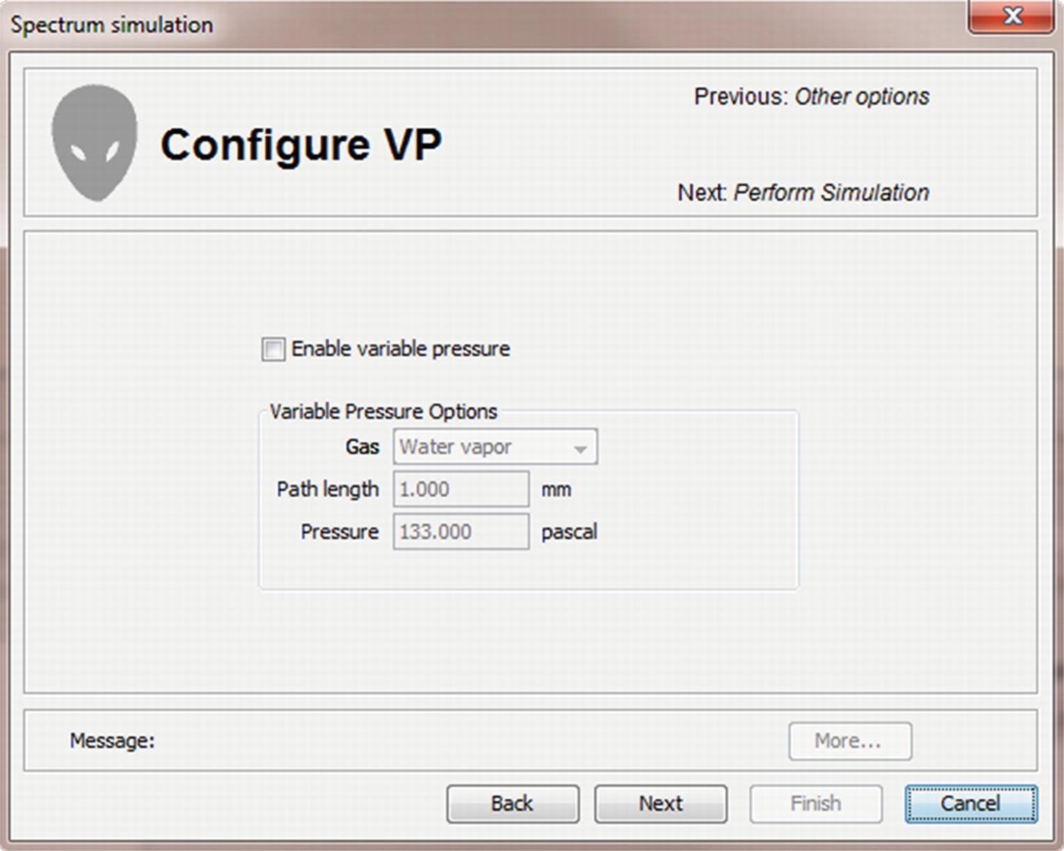
Menu for selection of variable pressure SEM operating conditions

The “configure VP” page provides an advanced option to simulate the beam scatter in a variable-pressure or environmental SEM. If the check box is selected, you may select a gas (“water,” “helium,” “nitrogen,” “oxygen” or “argon”), a gas path length and a nominal pressure. The gas path length is the distance from the final pressure limiting aperture to the sample. 1 Torr is equivalent to 133 Pa (◘ Figs. 17.40 and 17.41).

Fig. 17.40

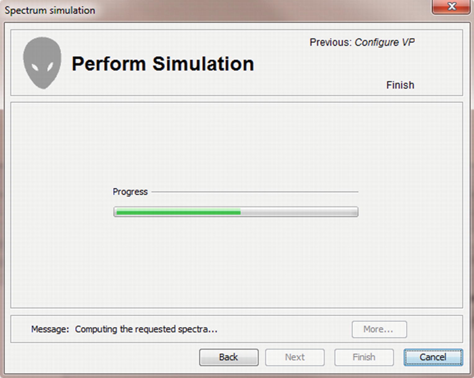
The “perform simulation” page shows progress as the electron trajectories are simulated. When the simulation is complete the “finish” button will enable to allow you to close the dialog

Fig. 17.41

Simulation results: X-ray spectrum

The primary output of a simulation is a spectrum. The simulated spectrum looks and acts to the best of our ability to simulate measured spectra like a spectrum collected from the specified material under the specified conditions on the specified detector. You can treat simulated spectra like measured spectra in the sense that you can simulate an “unknown” standards and reference spectra and quantify the “unknown” as though it had been measured (◘ Fig. 17.42).

Fig. 17.42

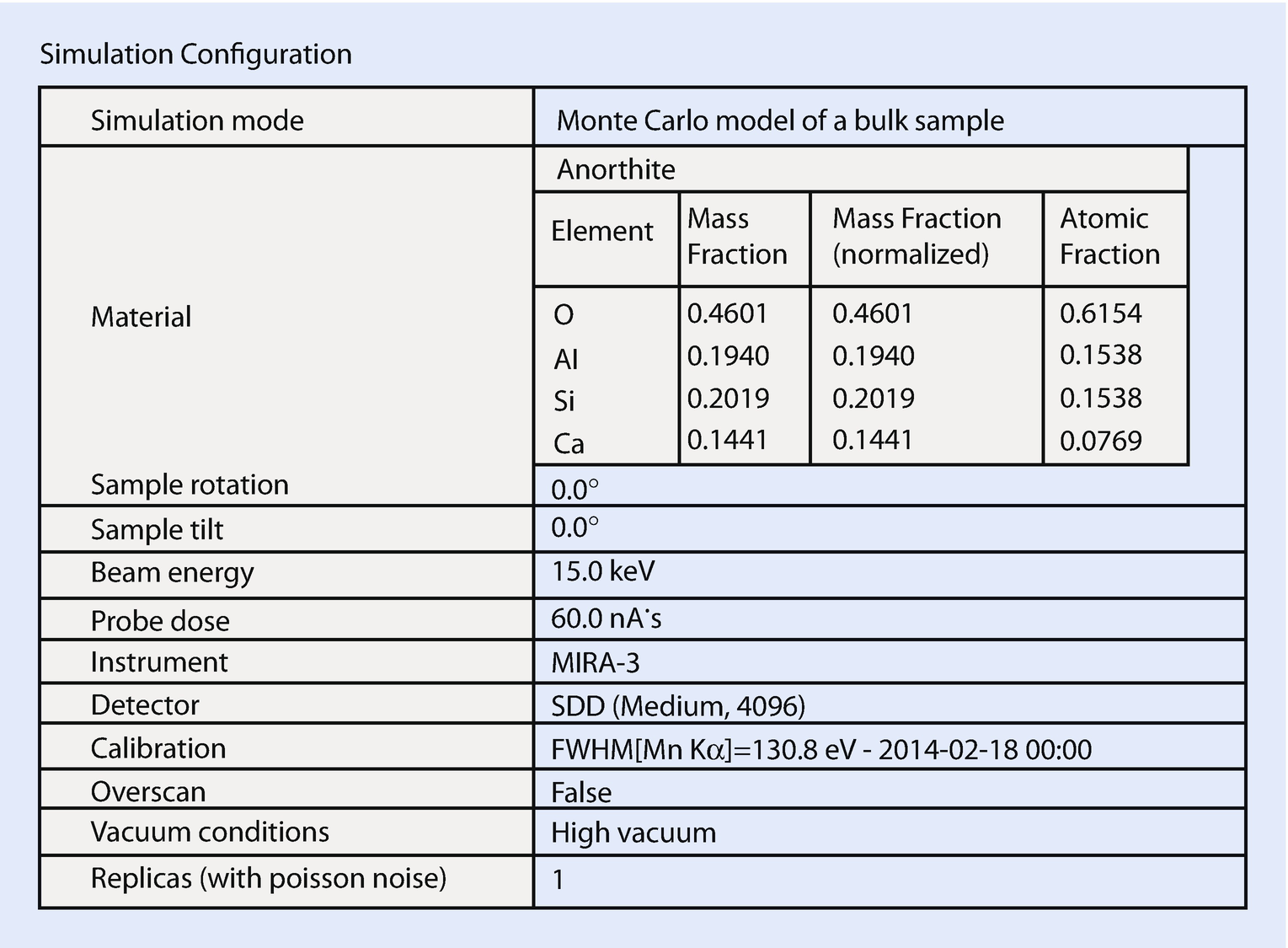
Simulation results: configuration record

The report tab contains additional details about the simulation including configuration and results information. The first table summarizes the simulation configuration parameters. This table is available for all simulation modes (◘ Fig. 17.43).

Fig. 17.43

Simulation results: table of X-ray intensities from various sources

The “simulation results” table contains additional details derived from the simulation. The first two lines contain links to the simulated spectrum and a Virtual Reality Markup Language (VRML) representation of the sample and electron trajectories. The subsequent rows contain raw data detailing the generation and emission of various different kinds of characteristic X-rays. Only those modes which were selected will be available. The generated X-rays column tabulates the relative number of X-rays generated within the sample and emitted into a milli-steradian. The emitted column tabulates the X-rays that are generated and also escape the sample in the direction of the detector. The ratio is the fraction of generated X-rays that escape the sample in the direction of the detector. The final rows compare the relative amount of characteristic fluorescence to the amount of primary characteristic and bremsstrahlung emission (◘ Fig. 17.44).

Fig. 17.44

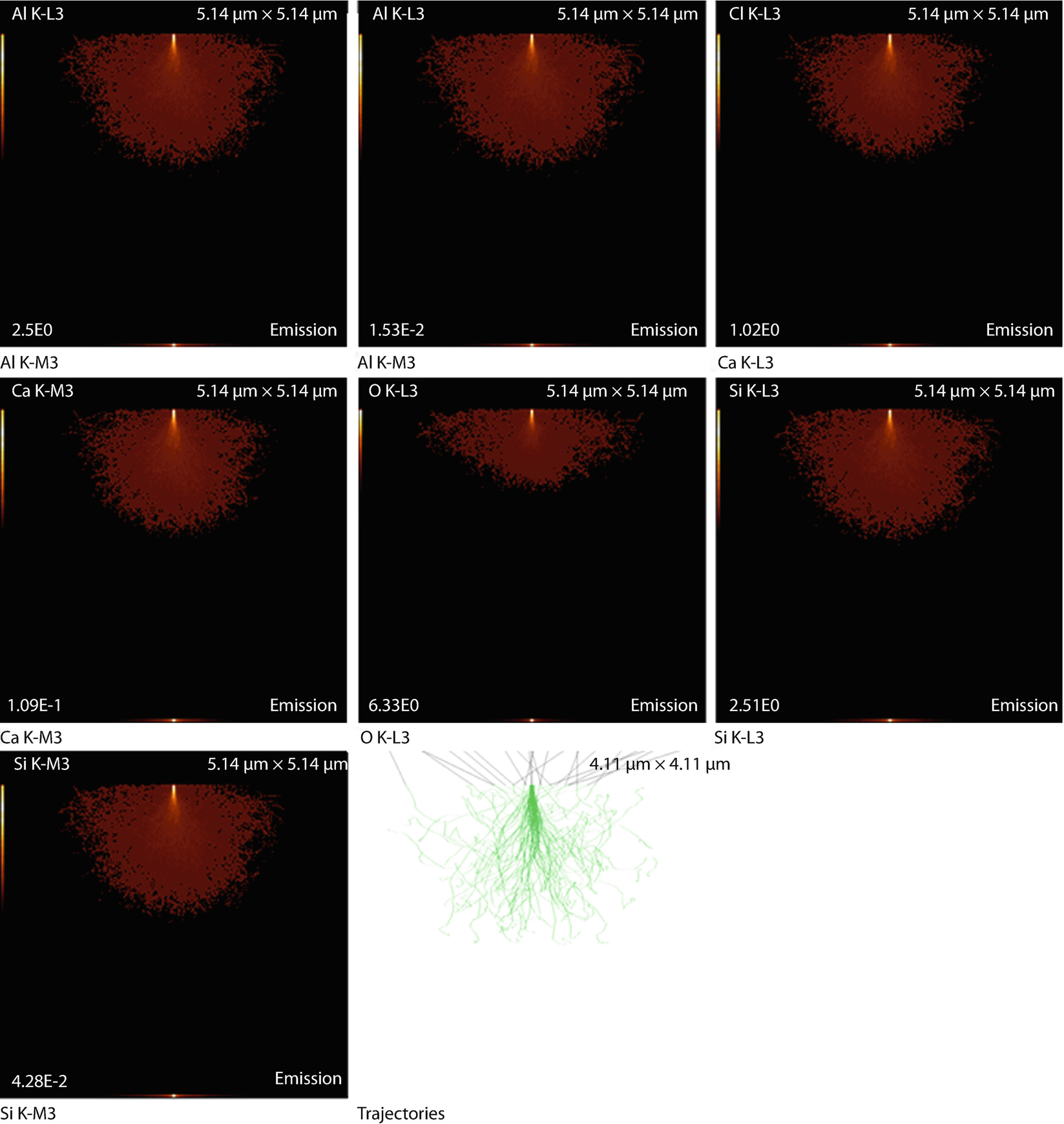
Simulation results: X-ray emission images and trajectories

The emission images show where the measured X-rays were generated. Because the images only display X-rays that escape the sample, the distinction between the strongly absorbed X-rays like the O K-L3 (Kα) and the less strongly absorbed like the Si K-L3 (Kα) is evidenced by the flattened emission profile in the Si K-L3 image. The last image shows the first 100 simulated electron trajectories (down to a kinetic energy of 50 eV.) The color of the trajectory segment varies as the electron passes through the different materials present in the sample. The gray lines exiting the top of the image are backscattered electrons (trajectories in vacuum).

17.2.4 Optional Tables

The “Fractional Emission Depths and Volumes” Table (◘ Fig. 17.45)

Fig. 17.45

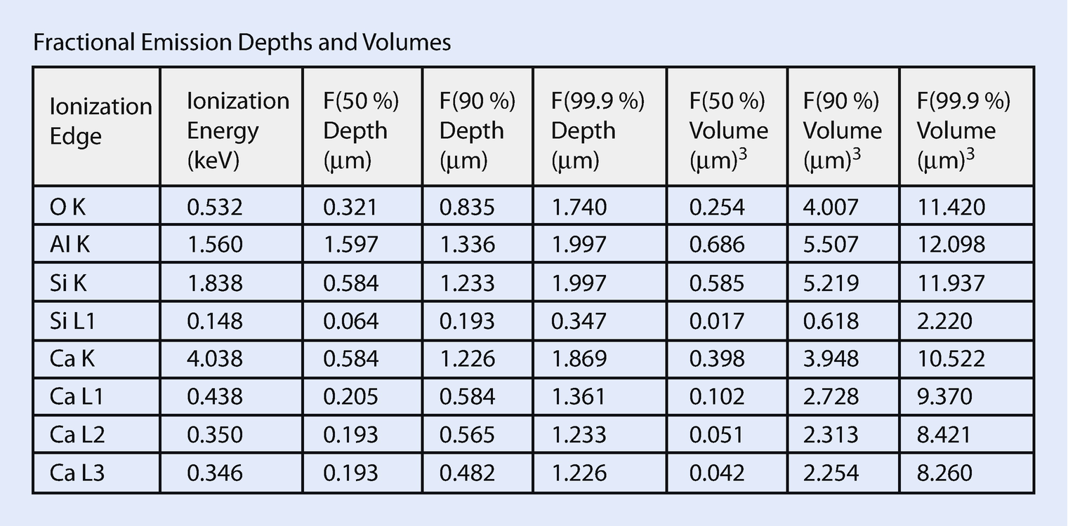
Output table listing depth and volumes from which 50 % or 90 % of the measured X-rays are emitted

When simulating a bulk sample, an additional report table shows the depth and the volumes from which 50 % or 90 % of the measured X-rays are emitted. The depth and volume are largely determined by the ionization edge energy and X-ray absorption. Low ionization edge energies emit from larger volumes but lower energy X-rays also tend to be more strongly absorbed.

17.2.4.1 The “VP Scatter Data” Table

In variable pressure mode, the gas in the chamber can scatter the incident electrons before they strike the sample. Despite the fact that these scatters tend to be small angle events, the path length is relatively long and electrons can scatter hundreds of microns to millimeters. The consequence can be demonstrated by simulating a moderate sized inclusion, shown in ◘ Fig. 17.46. In simulated high-vacuum mode, the excitation volume remains entirely within the inclusion. In simulated variable-pressure mode, the electrons can scatter out of the beam, entirely missing the inclusion and striking the surrounding matrix.

Fig. 17.46

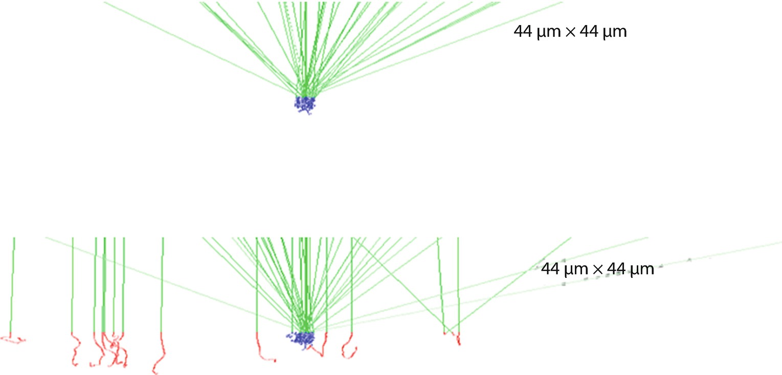
(upper) Simulated trajectories for high-vacuum conditions. All the electrons strike the inclusion. (lower) Trajectories simulated for variable pressure mode with 1-mm gas path length through water vapor at 133 Pa. The green trajectories are the incident and backscattered electrons

One way to understand the scatter is to consider a series of concentric rings on the surface of the sample centered at the beam axis. The “VP Scatter Data” table (◘ Fig. 17.47), summarizes the number and number fraction of the incident electrons which intersect the various rings. In this simulation, 87 % of the initial electrons are undeflected. However, at least one electron (0.1 %) is scattered further than 700 μm and 1.2 % are scattered more than 50 μm. This qualitative information is useful because it gives us a sense of how significant beam scatter will be in variable pressure mode. It gives a sense of whether true quantitative analysis is possible and how much of an error will be introduced by the beam scatter. The consequences are evident in the spectrum from an inclusion of admiralty brass in an aluminum. The aluminum is present in significant quantities in the variable pressure mode acquisition.

Fig. 17.47

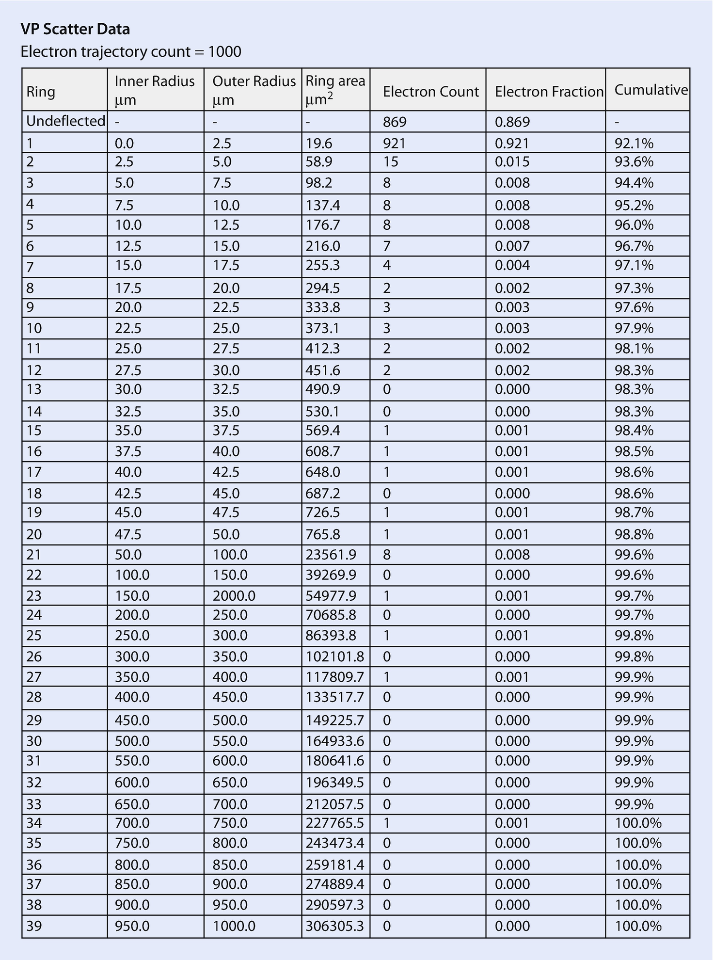
Distribution of gas-scattered electrons into a series of concentric rings

◘ Figure 17.48 shows EDS spectra calculated for a brass inclusion in an aluminum matrix under VPSEM (red) and conventional vacuum (blue) operation. The large peak for Al under VPSEM conditions reveals the extent of gas scattering outside the focused beam. Interestingly, the Al is not zero in the “high-vacuum” spectrum because of continuum generated secondary fluorescence. Increasing the size of the inclusion does not eliminate the slight Al peak but turning off the simulation of continuum fluorescence does.

Fig. 17.48

Comparison of spectra calculated for a brass inclusion in aluminum: VPSEM (red) and conventional vacuum (blue) operation. 1-mm gas path length through water vapor at 133 Pa

Open Access This chapter is licensed under the terms of the Creative Commons Attribution-NonCommercial 2.5 International License (http://creativecommons.org/licenses/by-nc/2.5/), which permits any noncommercial use, sharing, adaptation, distribution and reproduction in any medium or format, as long as you give appropriate credit to the original author(s) and the source, provide a link to the Creative Commons license and indicate if changes were made.

The images or other third party material in this chapter are included in the chapter's Creative Commons license, unless indicated otherwise in a credit line to the material. If material is not included in the chapter's Creative Commons license and your intended use is not permitted by statutory regulation or exceeds the permitted use, you will need to obtain permission directly from the copyright holder.

References

1. Pouchou J-L, Pichoir P (1991) “Quantitative analysis of homogeneous or stratified microvolumes applying the model PAP”. In: Heinrich K, Newbury D (eds) Electron Probe Quantitation. New York: Plenum, p163Crossref
2. Ritchie N (2009) Spectrum simulation in DTSA-II. Microsc Microanal 15:454Crossref
3. Ritchie N (2010) Using DTSA-II to simulate and interpret energy dispersive spectra from particles. Microsc Microanal 16:248Crossref
4. Ritchie N (2011a) “Getting Started with NIST DTSA-II.” In: Lyman C (ed) Microscopy Today. Cambridge Univ. Press. 19(1):26
5. Ritchie N (2011b) “Manipulating Spectra with DTSA-II.” In: Lyman C (ed) Microscopy Today. Cambridge Univ. Press. 19(3):34Crossref
6. Ritchie N (2011c) “Standards-Based Quantification in DTSA-II – Part I.” In: Lyman C (ed) Microscopy Today. Cambridge Univ. Press. 19(5):30
7. Ritchie N (2012) “Standards-Based Quantification in DTSA-II – Part II.” In: Lyman C (ed) Microscopy Today. Cambridge Univ. Press. 20(1):14
8. Ritchie N (2017a) “DTSA-II, a multiplatform software package for quantitative x-ray microanalysis.” Available free at the National Institute of Standards and Technology website (search “DTSA-II”): ► http://​www.​cstl.​nist.​gov/​div837/​837.​02/​epq/​dtsa2/​index.​html
9. Ritchie N (2017b) “Efficient simulation of secondary fluorescence Via NIST DTSA-II Monte Carlo” Microsc Microanal 23:618Crossref

Footnotes

1

Don’t worry if you don’t understand the difference between a reference and a standard spectrum. This will be explained later.