Attempting Electron-Excited X-Ray Microanalysis in the Variable Pressure Scanning Electron Microscope (VPSEM)

While X-ray analysis can be performed in the Variable Pressure Scanning Electron Microscope (VPSEM), it is not possible to perform uncompromised electron-excited X-ray microanalysis. The measured EDS spectrum is inevitably degraded by the effects of electron scattering with the atoms of the environmental gas in the specimen chamber before the beam reaches the specimen. The spectrum is always a composite of X-rays generated by the unscattered electrons that remain in the focused beam and strike the intended target mixed with X-rays generated by the gas-scattered electrons that land elsewhere, micrometers to millimeters from the microscopic target of interest.

It is critical to understand how severely the measured spectrum is compromised, what strategies can be followed to minimize these effects, and what “workarounds” can be applied in special circumstances to solve practical problems. The impact of gas-scattered electrons on the legitimacy of the analysis depends on the exact circumstances of the VPSEM conditions (beam energy, gas species, path length through the gas) and the characteristics of the specimen and its surroundings. Gas scattering effects increase in significance as the constituent(s) of interest range in concentration from major (concentration C > 0.1 mass fraction) to minor (0.01 ≤ C ≤ 0.1) to trace (C < 0.01).

25.1 Gas Scattering Effects in the VPSEM

The VPSEM allows operation with elevated gas pressure in the specimen chamber, typically 10 Pa to 1000 Pa but even higher in the “environmental SEM” (ESEM), where pressures of 2500 Pa are possible, permitting liquid water to be maintained in equilibrium when the specimen is cooled to ~ 3 °C. Such specimen chamber pressures are several orders of magnitude higher than that of a conventional high-vacuum SEM, which typically operates at 10⁻² Pa to 10⁻⁴ Pa or lower. As the beam emerges from the high vacuum of the electron column through the final aperture into the elevated pressure of the specimen chamber, elastic scattering events with the gas atoms begin to occur. Although the volume density of the gas atoms in the chamber is very low compared to the density of a solid material, the path length that the beam electrons must travel typically ranges from 1 mm to 10 mm or more before reaching the specimen. As illustrated in ◘ Fig. 25.1, when elastic scattering occurs along this path, the angular deviation causes beam electrons to substantially deviate out of the focused beam creating a “skirt.” The unscattered beam electrons follow the expected path defined by the objective lens field and land in the focused beam footprint identical to the situation at high vacuum but with reduced intensity due to the gas scattering events that rob the beam of electrons. The electrons that remain in the beam behave exactly as they would in a high vacuum SEM, creating the same interaction volume and generating X-rays with exactly the same spatial distribution to produce identically the same spectrum. This “ideal” high vacuum equivalent spectrum represents the true microanalysis condition. However, this ideal spectrum is degraded by the remotely scattered electrons in the skirt which generate characteristic and continuum (bremsstrahlung) X-rays from whatever material(s) they strike.

../images/271173_4_En_25_Chapter/271173_4_En_25_Fig1_HTML.png — Fig. 25.1
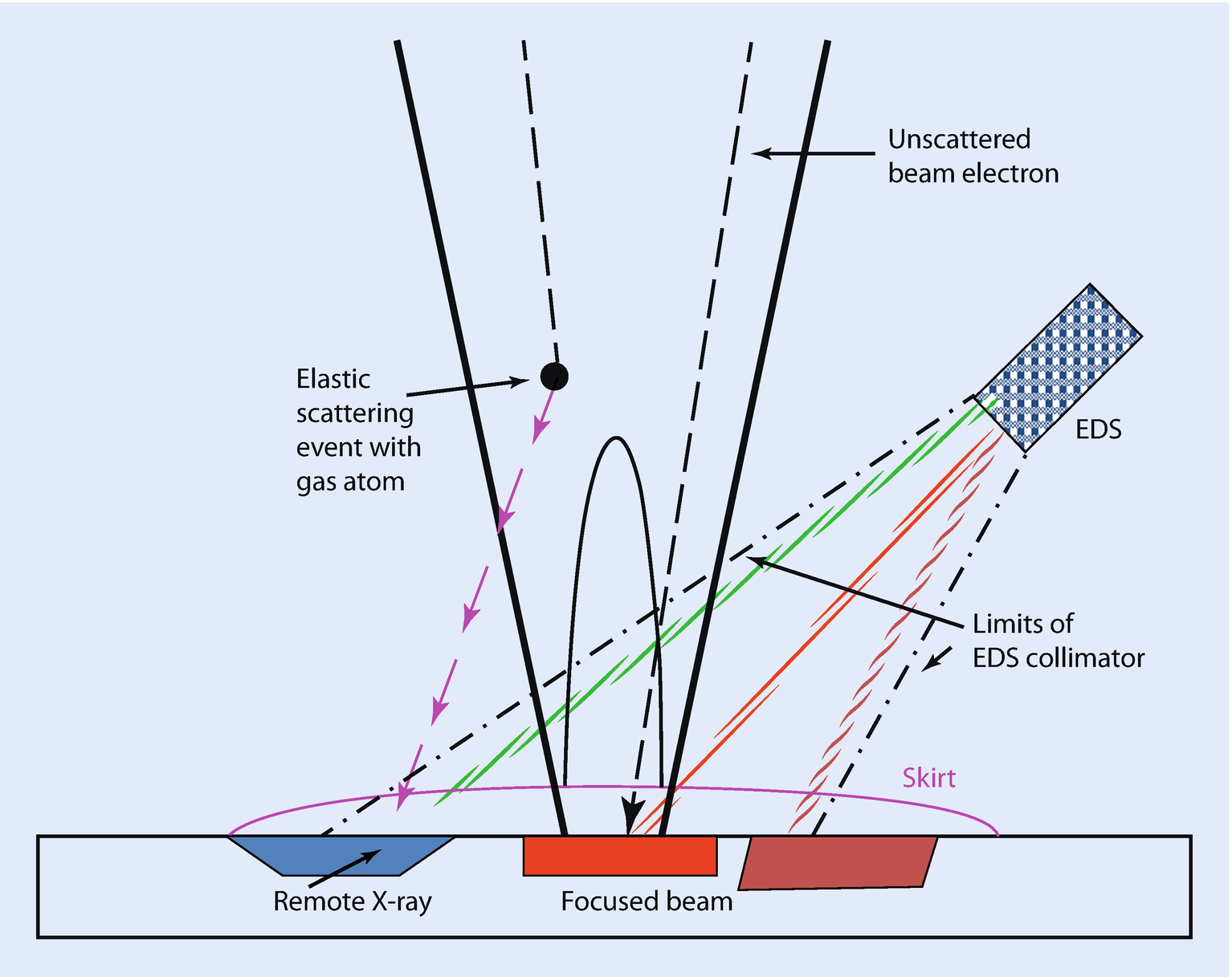
Schematic diagram of gas scattering in a VPSEM

The extent of the beam skirt can be estimated from the ideal gas law (the density of particles at a pressure p is given by n/V = p/RT, where n is the number of moles, V is the volume, R is the gas constant, and T is the temperature) and by assuming single-event elastic scattering (Danilatos 1988):

${R}_s=\left(0.364\ Z/E\right)\ {\left(p/T\right)}^{1/2}{L}^{3/2}x$

(25.1)

R _s = skirt radius (m)
Z = atomic number of the gas
E = beam energy (keV)
p = pressure (Pa)
T = temperature (K)
L = path length in gas (m) (GPL)

◘ Figure 25.2 plots the skirt radius for a beam energy of 20 keV as a function of the gas path length through oxygen at several different chamber pressures. For a pressure of 100 Pa and a gas path length of 5 mm, the skirt radius is calculated to be 30 μm. Consider the change in scale due to gas scattering. The high vacuum microanalysis footprint can be estimated with the Kanaya-Okayama range equation. For a copper specimen and E ₀ = 20 keV, the full range R _K-O = 1.5 μm, which is a good estimate of the diameter of the interaction volume projected on the entrance surface, the “microanalysis footprint.” The gas scattering skirt is thus a factor of 40 larger in diameter, but a factor of 1600 larger in area.

../images/271173_4_En_25_Chapter/271173_4_En_25_Fig2_HTML.png — Fig. 25.2
Radial dimension of gas scattering skirt as a function of gas path length at various pressures for O₂ and E ₀ = 20 keV

While Eq. (25.1) is useful to estimate the extent of the gas scattering on the spatial resolution of X-ray microanalysis under VPSEM conditions, it provides no information on the relative fractions of the spectrum that arise from the unscattered beam electrons (exactly equivalent to the high vacuum microanalysis footprint) and the skirt. The Monte Carlo simulation embedded in NIST DTSA-II enables explicit treatment of gas scattering to provide detailed information on the unscattered beam electrons and the distribution of electrons scattered into the skirt. The VPSEM menu of DTSA-II is shown in ◘ Fig. 25.3 and allows selection of the gas path length, the gas pressure, and the gas species (He, N₂, O₂, H₂O, or Ar). An example of a portion of the electron scattering information produced by the Monte Carlo simulation is listed in ◘ Table 25.1 for a gas path length of 5 mm through 100 Pa of oxygen with a 20-keV beam energy; the full table extends to 1000 μm. This data set is plotted as the cumulative electron intensity as a function of radial distance out to 50 μm from the beam center in ◘ Fig. 25.4. For these conditions the unscattered beam retains 0.70 of the beam intensity that enters the specimen chamber. The skirt out to a radius of 30 μm contains a cumulative intensity of 0.84 of the incident beam current. To capture 0.95 of the total current for a 5-mm gas path length in 100 Pa of oxygen requires a radial distance of approximately 190 μm, as shown in ◘ Fig. 25.5, which plots the skirt distribution out to 1000 μm (1 mm). The strong effect of the gas path length on the skirt radius, which follows a 3/2 exponent in the scattering Eq. 25.1, can be seen in ◘ Fig. 25.5 in the plots for 3 mm, 5 mm, and 10 mm gas path lengths.

../images/271173_4_En_25_Chapter/271173_4_En_25_Fig3_HTML.jpg — Fig. 25.3
Selection of VPSEM gas parameters in DTSA-II for simulation

Table 25.1

Portion of the electron scattering table for VPSEM simulation. Note the unscattered fraction of the 20 keV beam, 0.701 (100 Pa, 5-mm gas path length, oxygen). The full table extends to 1000 μm

Ring	Inner radius, μm	Outer radius, μm	Ring area, μm²	Electron count	Electron fraction	Cumulative, %
Undeflected	–	–	–	701	0.701	–
1	0.0	2.5	19.6	755	0.755	75.5
2	2.5	5.0	58.9	23	0.023	77.8
3	5.0	7.5	98.2	11	0.011	78.9
4	7.5	10.0	137.4	10	0.010	79. 9
5	10.0	12.5	176.7	7	0.007	80.6
6	12.5	15.0	216.0	6	0.006	81.2
7	15.0	17.5	255.3	9	0.009	82.1
8	17.5	20.0	294.5	10	0.010	83.1
9	20.0	22.5	333.8	4	0.004	83.5
10	22.5	25.0	373.1	3i	0.003	83.8
11	25.0	27.5	412.3	6	0.006	84.4
12	27.5	30.0	451.6	4	0.004	84.8
13	30.0	32.5	490.9	6	0.006	85.4
14	32.5	35.0	530.1	2	0.002	85.6
15	35.0	37.5	569.4	2	0.002	85.8
16	37.5	40.0	608.7	3	0.003	86.1
17	40.0	42.5	648.0	4	0.004	86.5

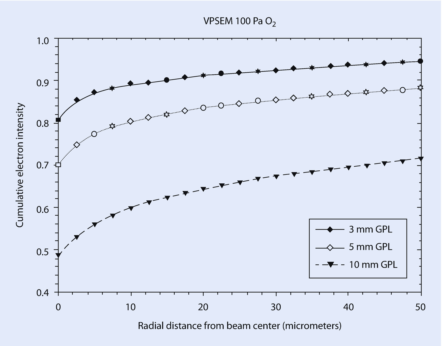
../images/271173_4_En_25_Chapter/271173_4_En_25_Fig4_HTML.png — Fig. 25.4
DTSA-II Monte Carlo calculation of gas scattering in a VPSEM: E ₀ = 20 keV; oxygen; 100 Pa; 3-, 5-, and 10-mm gas path lengths (GPL) to a radial distance of 50 μm

../images/271173_4_En_25_Chapter/271173_4_En_25_Fig5_HTML.png — Fig. 25.5
DTSA-II Monte Carlo calculation of gas scattering in a VPSEM: E ₀ = 20 keV; oxygen; 100 Pa; 3-, 5-, and 10-mm gas path lengths to a radial distance of 1000 μm

The extent of the degradation of the measured EDS spectrum by gas scattering is illustrated in the experiment shown in ◘ Fig. 25.6. The incident beam is placed at the center of a polished cross section of a 40 wt % Cu – 60 wt % Au alloy wire 500 μm in diameter surrounded by a 2.5-cm-diameter Al disk. For a beam energy of 20 keV and a gas path length of 4 mm through water vapor, the EDS spectra measured over a pressure range from 53 Pa to 1600 Pa are superimposed, showing the in-growth of the Al peak with increasing pressure. Even at 53 Pa, a detectable Al peak is observed, despite the beam center being 250 μm away from the Al. As the pressure is increased, the Al peak ranges from an apparent trace to minor and finally major constituent peak.

../images/271173_4_En_25_Chapter/271173_4_En_25_Fig6_HTML.jpg — Fig. 25.6
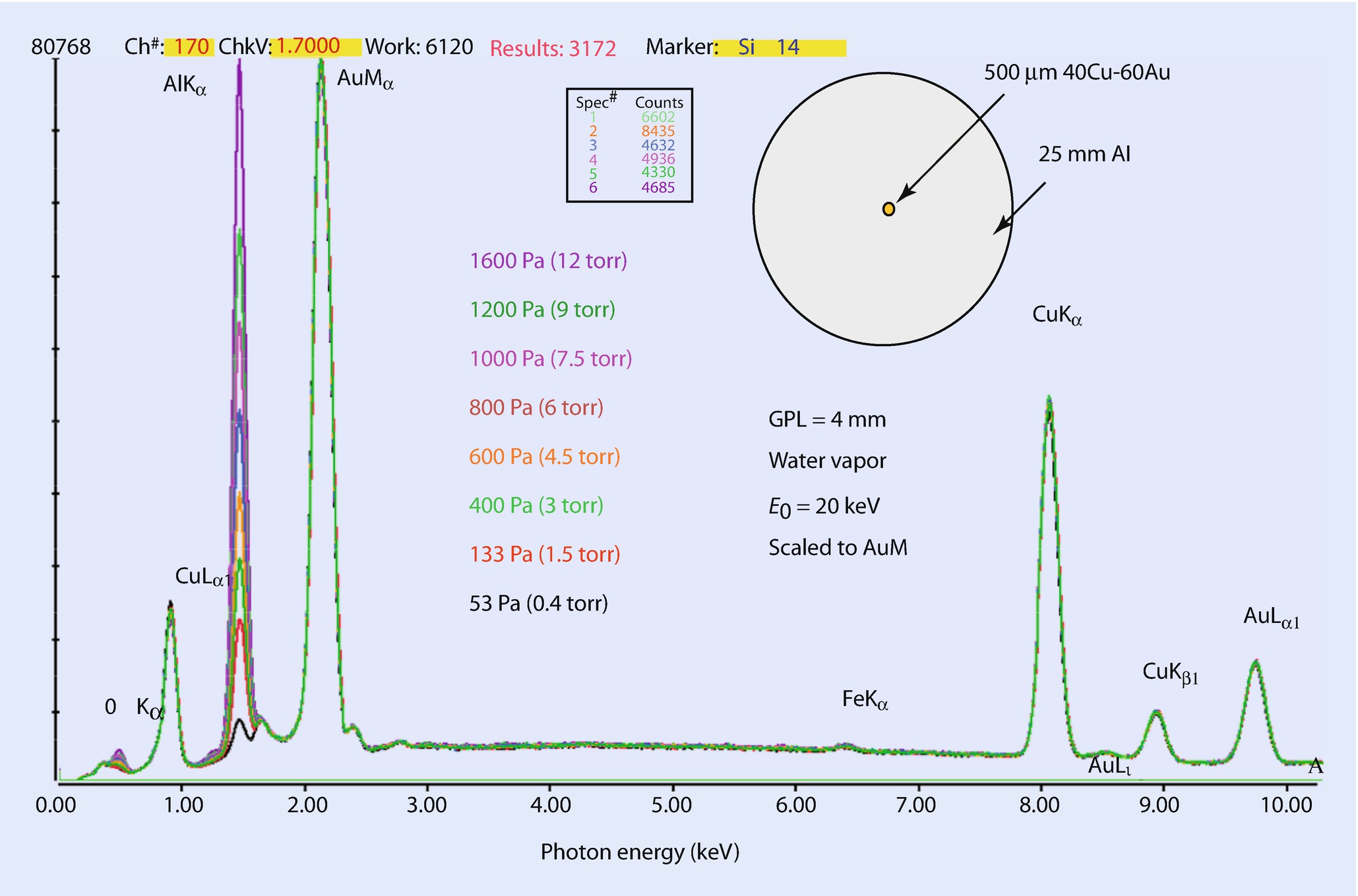
EDS spectra measured with the beam placed in the center of a 500 μm diameter wire of 40 wt % Cu–60 wt %Au surrounded by a 2.5-cm-diameter Al disk; E ₀ = 20 keV; gas path length = 4 mm; oxygen at various pressures

DTSA-II also simulates the composite spectrum created by these two classes of electrons as they strike the specimen. Various configurations of two different materials can be specified, one that the unscattered beam strikes, for example, a particle, and the other by the skirt electrons, for example, the surrounding matrix. ◘ Figure 25.7 shows spectra simulated for the example of ◘ Fig. 25.6, the 500-μm-diameter 40 wt %Cu–60 wt %Au wire in the Al disk with a 4-mm-gas path length through water vapor. The simulation of the lowest VPSEM gas pressure of 53 Pa produces a low level Al peak similar to the experimental measurement. Thus, even at this low pressure and short gas path length for which 89 % of the electrons remain in the focused beam, there are still gas-scattered electrons falling at least 250 μm from the beam impact. As the pressure is progressively increased, the in-growth of the Al peak due to the skirt electrons is well modeled by the Monte Carlo simulation.

../images/271173_4_En_25_Chapter/271173_4_En_25_Fig7_HTML.jpg — Fig. 25.7
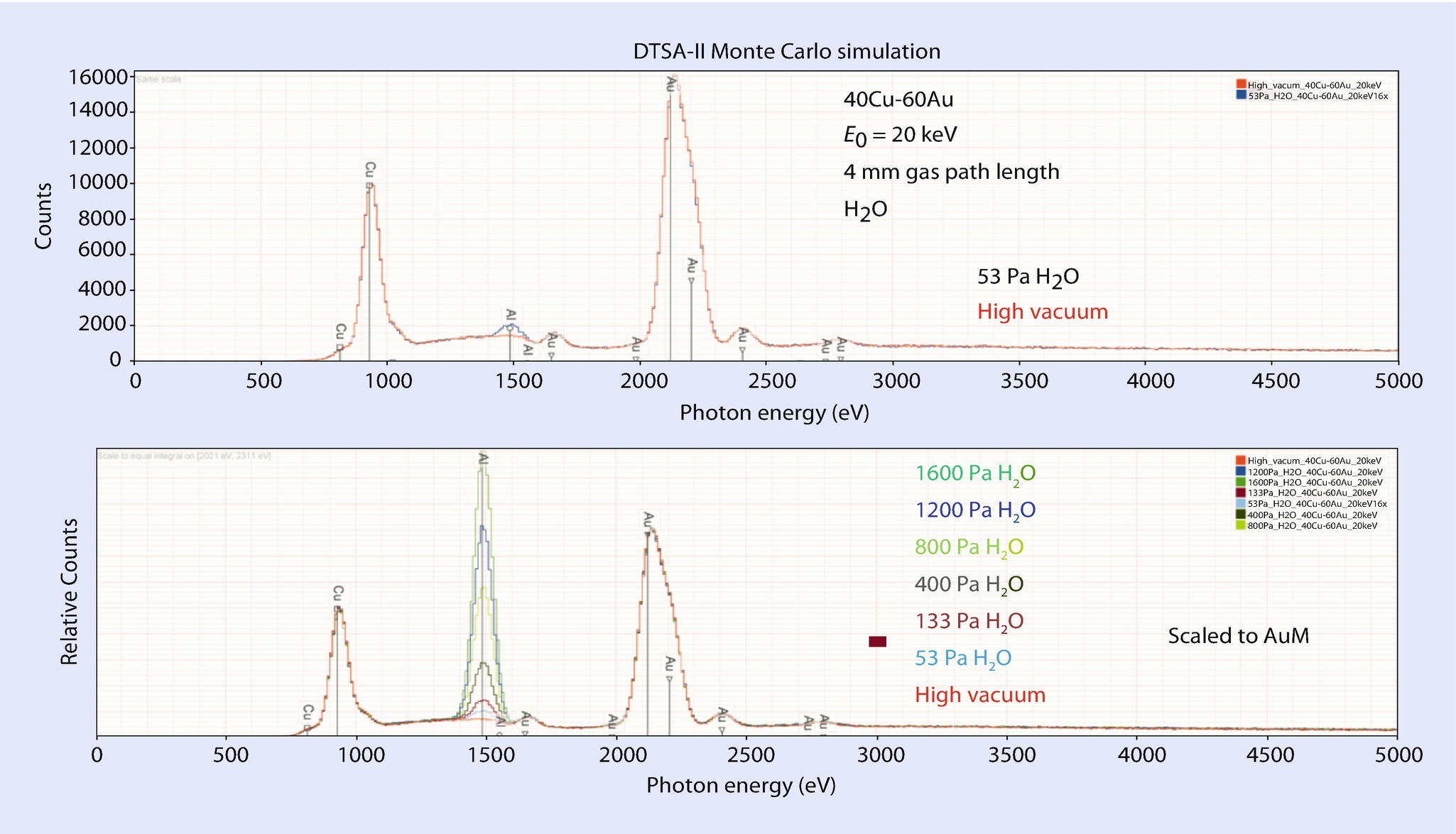
DTSA-II Monte Carlo simulations of the specimen and gas scattering conditions of ◘ Fig. 25.6. Upper plot: high vacuum and 53 Pa (4 mm GPL, H₂O). Lower plot: high vacuum and various pressures from 53 Pa to 1600 Pa

25.1.1 Why Doesn’t the EDS Collimator Exclude the Remote Skirt X-Rays?

Gas scattering in the VPSEM mode always degrades the incident beam, transferring a significant fraction of the beam electrons into the skirt. The radius of the skirt can reach a millimeter or more from the focused beam impact. It might be thought that the EDS collimator would restrict the acceptance area of the EDS to exclude most of the skirt. As shown in the schematic diagram in ◘ Fig. 25.8, while a simple collimator acts to successfully shield the EDS from accepting X-rays produced by backscattered electrons striking the lens and chamber walls, the acceptance volume near the column optic axis is quite large. The EDS acceptance is not defined by looking back at the detector from the specimen space as the cone of rays whose apex is at the beam impact on the specimen and whose base is the detector active area (the dashed red lines in ◘ Fig. 25.8). While the red lines define the solid angle of the detector for emission from the beam impact point, the acceptance region is actually defined by looking from the detector through the collimator at the specimen space (the dashed green lines in ◘ Fig. 25.8). The true area of acceptance can be readily determined by conducting X-ray mapping measurements. ◘ Fig. 25.9 shows a series of measurements of X-ray maps of a machined Al disk taken at the lowest available magnification (largest scan field) over a series of working distances. The false color scale shows the while the intensity is not uniform within a map, it generally varies by less than 30 % over the full map, a distance of millimeters, and moreover, as the maps are measured at different working distances, there is only about 30 % variation over the vertical range, which is confirmed by the plot of the intensity measured at the center of each map. Thus, X-rays generated throughout a large volume are accepted through the collimator by the EDS so that collimation provides virtually no relief from the effects of remote X-ray generation caused by gas scattering in the VPSEM.

../images/271173_4_En_25_Chapter/271173_4_En_25_Fig8_HTML.png — Fig. 25.8
Schematic diagram showing the acceptance area of the EDS collimator

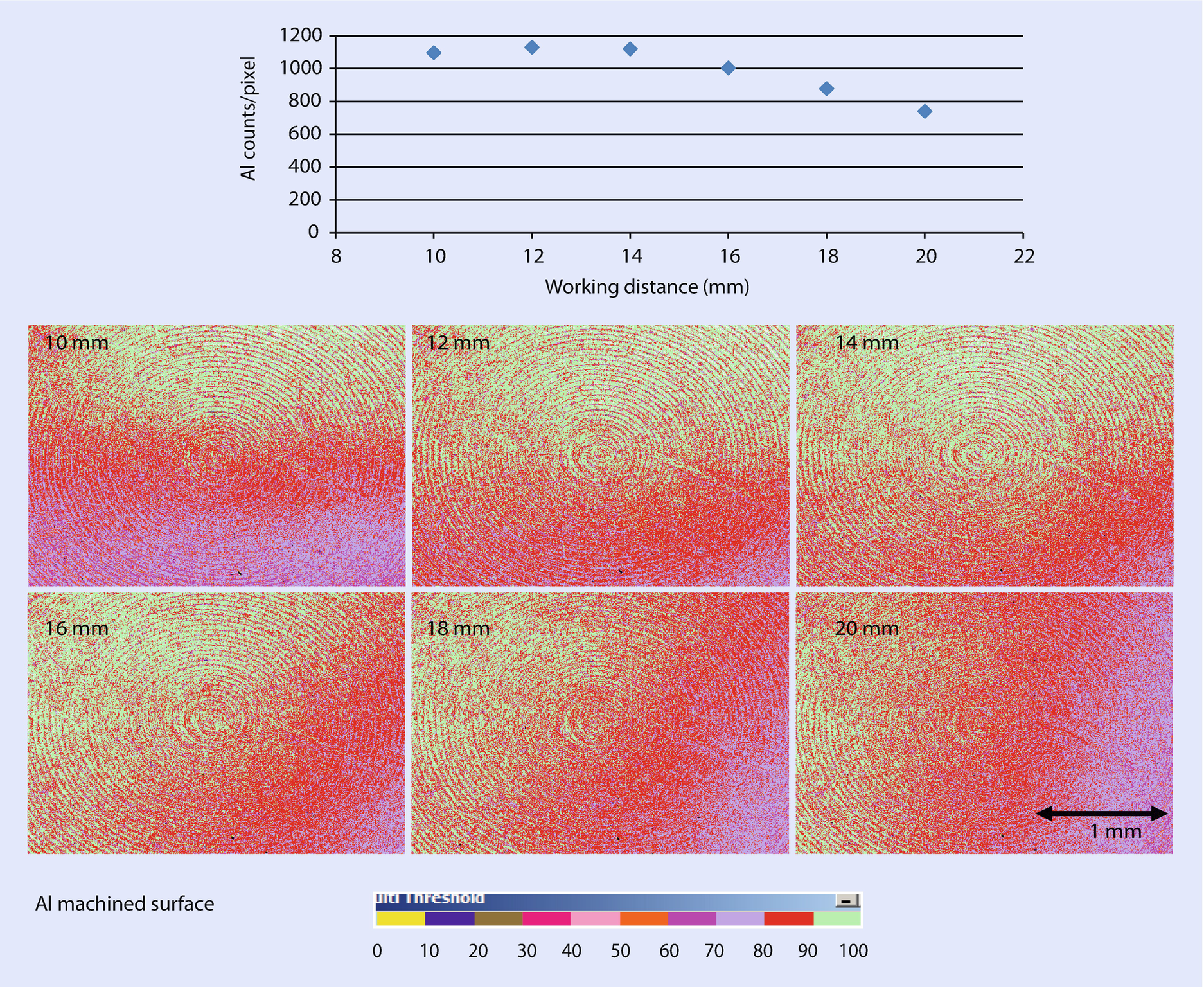
../images/271173_4_En_25_Chapter/271173_4_En_25_Fig9_HTML.png — Fig. 25.9
Collimator acceptance volume as determined by mapping an Al disk at various working distances (10–20 mm) at the widest scanned field (i.e., lowest magnification); the plot shows the intensity measured at the center of the scan field as a function of working distance

25.1.2 Other Artifacts Observed in VPSEM X-Ray Spectrometry

Inelastic scattering of the beam electrons and backscattered electrons with the atoms of the environmental gas causes inner shell ionization leading to X-ray emission that contributes to the measured spectrum. The density of gas atoms (number/unit volume) is orders of magnitude lower than the density in the solid specimen, but the distance that the beam travels in the gas is orders of magnitude longer than it travels in the solid. The contribution of the environmental gas is illustrated for a simple experiment in ◘ Fig. 25.10, where the beam strikes a carbon target at a series of different pressures. The in-growth of the oxygen peak from ionization of the water vapor used as the environmental gas can be seen. A detectable oxygen peak is seen for pressures of 133 Pa (1 torr) and higher for this particular gas path length (6 mm) and beam energy (20 keV). ◘ Figure 25.11 shows an example of the contribution of the environmental gas to the spectrum measured from a 50 μm diameter glass shard with the composition listed in the figure placed on a carbon substrate. At the lower pressure (266 pA = 2 torr) for the gas path length used (3 mm), the footprint of the focused beam and skirt remain within the 50 μm diameter glass shard, as evidenced by the negligible C intensity in the spectrum. An O peak is also observed, at least some of which is actually from the specimen. When the pressure is increased by a factor of five to 1330 Pa (10 torr), the C intensity rises significantly because the skirt now extends beyond the boundary of the particle, and the O peak intensity increases by a factor of four, all of which is due to the environmental gas. It is also worth noting that in addition to characteristic X-rays from the environmental gas, there is increased bremsstrahlung generation as well from the inelastic scattering of beam and backscattered electrons with the gas atoms. In ◘ Fig. 25.11, the background is substantially higher for the spectrum measured at the elevated pressure, leading to a reduced peak-to-background, which is easily seen for the Zn L-family and Al K-L₂ peaks, an effect which makes for poorer limits of detection.

../images/271173_4_En_25_Chapter/271173_4_En_25_Fig10_HTML.png — Fig. 25.10
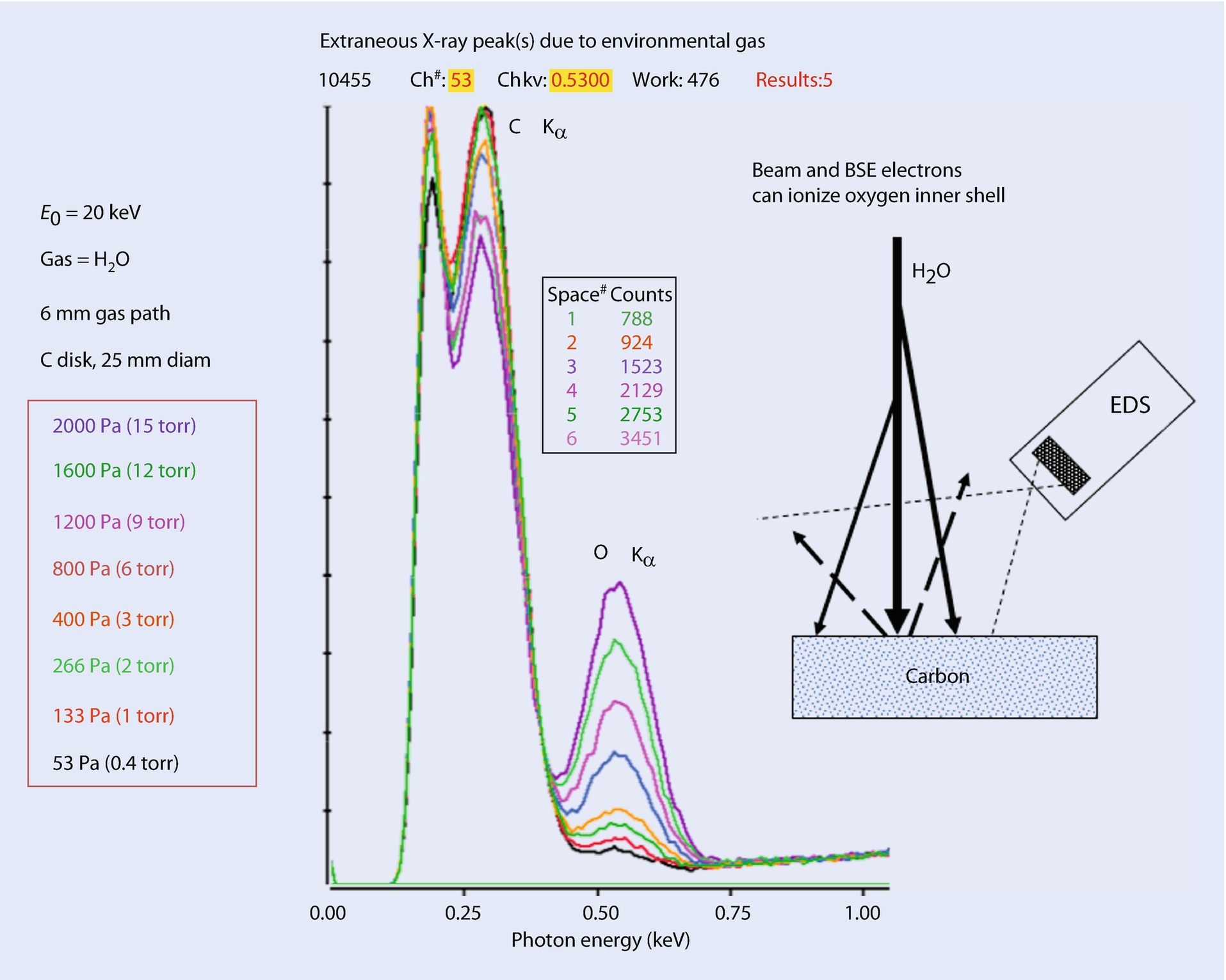
Generation of O K X-rays from the environmental gas as a function of chamber pressure

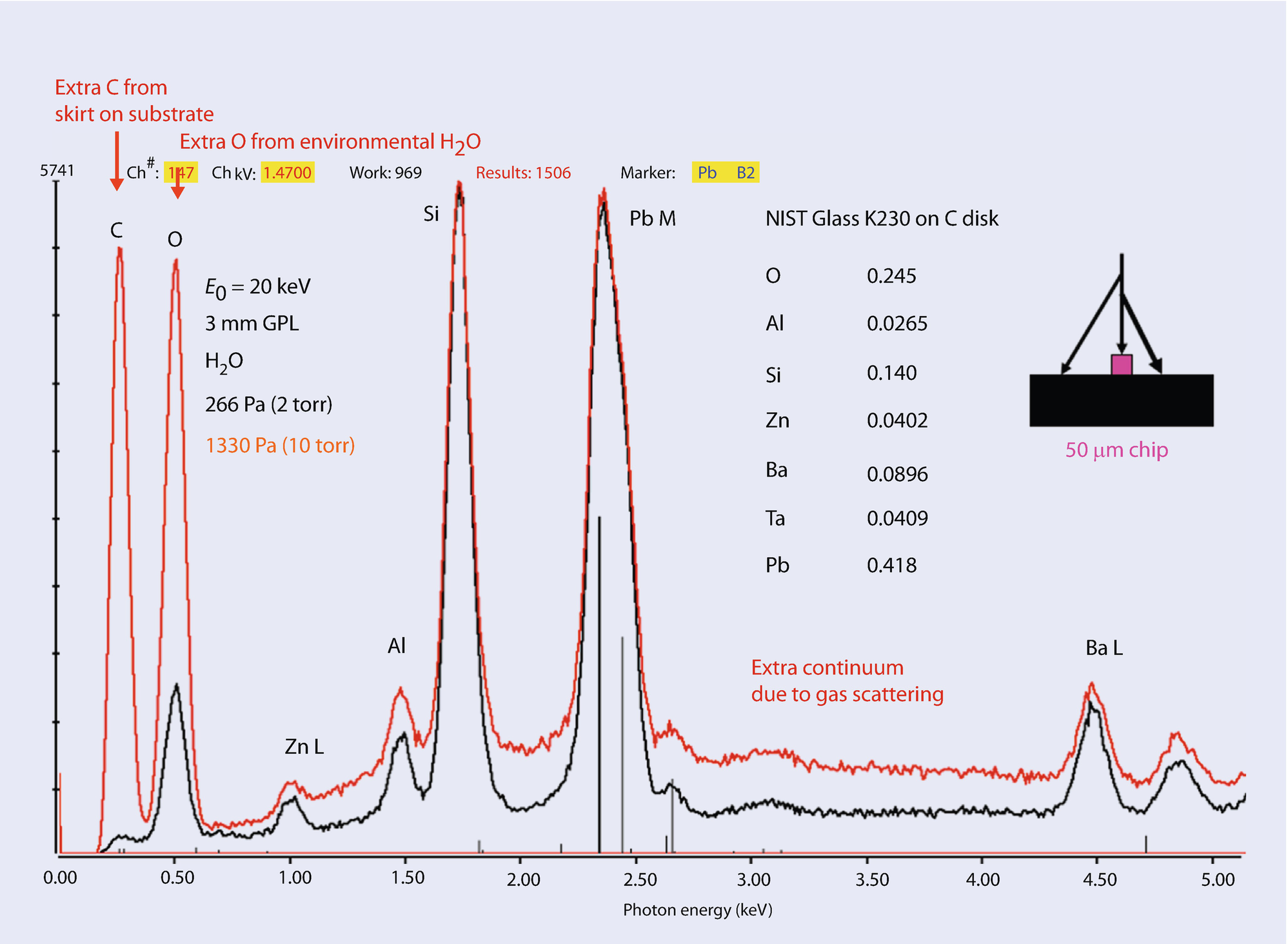
../images/271173_4_En_25_Chapter/271173_4_En_25_Fig11_HTML.png — Fig. 25.11
Modification of the measured X-ray spectrum by gas scattering, including in-growth of the O K peak from contributions of the environmental gas as well as increased background due to increased *bremsstrahlung* created by the gas scattering

If the environmental gas can contribute to the spectrum, can the gas also absorb X-rays from the specimen? Because of the low gas density, this effect might be expected to be negligible, and as listed in ◘ Table 25.2, which is calculated for a 40 –mm-path through the gas from the X-ray source at the beam impact on the specimen to the EDS, for the lowest pressure considered, 10 Pa, over 99 % of the X-rays of all energies leaving the specimen in the direction of the detector arrive there, even for F K, the energy of which, 0.677 keV, is just above the O K-shell absorption energy, 0.535 keV, which results in a large mass absorption coefficient. When the pressure is increased to 100 Pa, the loss of F K due to absorption increases to ~ 6 %, and at a pressure of 2500 Pa (18.8 torr), ~ 80 % of the F K radiation is lost to gas absorption, and even Al K-L₂ suffers a 20 % loss in intensity compared to the conventional high vacuum SEM situation.

Table 25.2

Absorption of X-rays by the environmental gas (O₂) (40-mm source to EDS)

Element/X-ray	I/I₀ (2500 Pa)	I/I₀ (100 Pa)	I/I₀ (10 Pa)
F K (0.677 keV)	0.194	0.940	0.994
NaK (1.041 keV)	0.572	0.979	0.998
AlK (1.487 keV)	0.805	0.992	0.9992
SiK (1.740 keV)	0.868	0.995	0.9995
S K (2.307 keV)	0.939	0.998	0.9998
ClK (2.622 keV)	0.957	0.998	0.9998
K K (3.312 keV)	0.986	0.999	0.9999
CaK (3.690 keV)	0.990	0.9996	0.9999

25.2 What Can Be Done To Minimize gas Scattering in VPSEM?

Manipulating the parameters in Eq. (25.1) provides the basis for minimizing, but not eliminating, the effects of gas scattering:

1.
Z, atomic number of the scattering gas: By lowering the atomic number of the gas, the skirt radius is reduced. This effect is illustrated in ◘ Fig. 25.12, which is derived from DTSA-II Monte Carlo simulations comparing the skirt radius for He and O₂ for a 10-mm gas path length and 100-Pa gas pressure with a beam energy E ₀ = 20 keV.
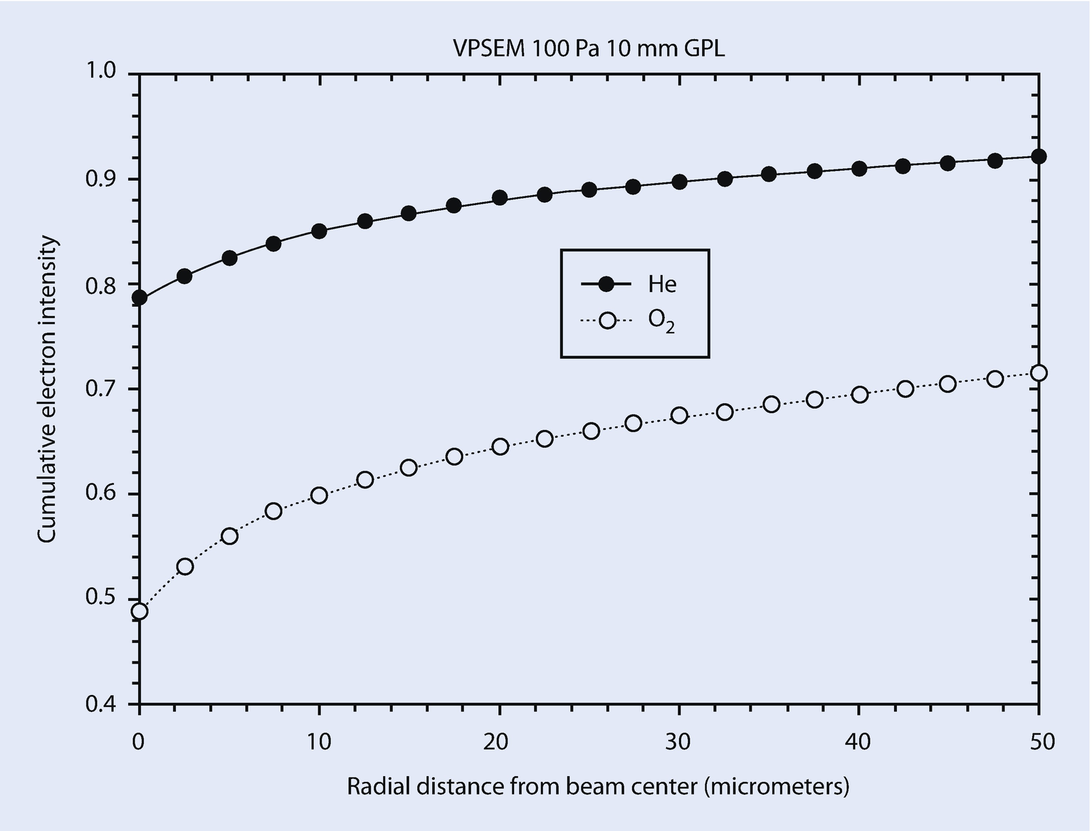Fig. 25.12
Comparison of the scattering skirt for He and O₂
2.
E, beam energy (keV). Operating at the highest possible beam energy reduces the gas scattering skirt.
3.
p, the gas pressure (Pa): Operating with the lowest possible gas pressure minimizes the gas scattering skirt
4.
T, the sample chamber temperature (K): The scattering skirt is reduced by operating at the lowest possible temperature.
5.
L, the gas path length (m). The shorter the gas path length, the smaller the gas scattering skirt, as shown in ◘ Fig. 25.4, where the skirt is compared for gas path lengths of 3 mm, 5 mm, and 10 mm. Note that the gas path length appears in Eq. (25.1) with a 3/2 power, so that the skirt radius is more sensitive to this parameter than the other parameters in Eq. (25.1). A modification to the vacuum system of the VPSEM that minimizes the gas path length consists of using a small diameter tube to extend the high vacuum of the electron column into the sample chamber.

25.2.1 Workarounds To Solve Practical Problems

Gas scattering effects can be minimized but not avoided, and for many VPSEM measurements and in situ experiments, the microscopist/microanalyst may be significantly constrained in the extent to which any of the parameters in Eq. (25.1) can actually be changed to reduce the gas scattering skirt without losing the advantages of VPSEM operation. The measured EDS spectrum is always compromised, but by carefully choosing the problems to study, successful X-ray analysis can still be performed. A useful way to consider the impact of gas scattering is the general concentration level at which the remote scattering corrupts the measured spectrum:

Major constituent: concentration C > 0.1 mass fraction
Minor constituent: 0.01 ≤ C ≤ 0.1
Trace constituent: C < 0.01

Depending on the exact nature of the specimen, gas scattering will almost always introduce spectral artifacts at the trace and minor constituent levels, and in severe cases artifacts will appear at the level of apparent major constituents.

25.2.2 Favorable Sample Characteristics

Given that the LVSEM operating conditions have been selected to minimize the gas scattering skirt, what specimen types are most likely to yield useful microanalysis results? If most of the gas scattering skirt falls on background material that contains an element or elements that are different from the elements of the target and of no interest, then by following a measurement protocol to identify the extraneous elements, the measured spectrum can still have value for identifying the elements within the target area, always recognizing that the target is being excited by the focused beam and the skirt.

25.2.2.1 Particle Analysis

Particle samples comprise a broad class of problems related to the environment, technology, forensics, failure analysis, and other areas. Particles are very often insulating in nature so that a conductive coating is required for examination in the conventional high vacuum SEM, and the complex morphologies of particles often make it difficult to apply a suitable coating. The VPSEM with its charge dissipation through gas ionization is an attractive alternative to achieve successful particle imaging. When VPSEM X-ray analysis measurements are needed to characterize particles, specimen preparation is critical to achieve a useful result. There are many methods available for particle preparation, but the general goal for successful VPSEM X-ray analysis is to broadly disperse the particles on a suitable substrate so that the unscattered beam and the innermost intense portion of the skirt immediately surrounding the beam can be placed on individual particles without exciting nearby particles. The more distant portions of the beam skirt may still excite other particles in the dispersion, but the relative fraction of the electrons that falls on these particles is likely to be sufficiently small that the artifacts introduced in the measured spectrum will be equivalent to trace (C < 0.01 mass fraction) constituents.

1.
When particles are collected on a smooth (i.e., not tortuous path) medium such as a porous polycarbonate filter, the loaded filter can be studied directly in the VPSEM with no preparation other than to attach a portion of the filter to a support stub. Prior to attempting X-ray measurements of individual particles, the X-ray spectrum of the filter material should be measured under the VPSEM operating conditions as the first stage of determining the analytical blank (that is, the spectral contributions of all the materials involved in the preparation except the specimen itself). In addition to revealing the elemental constituents of the filter, this blank spectrum will also reveal the contribution of the environmental gas to the spectrum.
2.
When particles are to be transferred from the collection medium, such as a tortuous path filter, or simply obtained from a loose mass in a container, the choice of the sample substrate is the first question to resolve. Conceding that VPSEM operation will lead to significant remote scattering that will excite the substrate, the sample substrate should be chosen to consist of an element that is not of interest in the analysis of individual particles. Carbon is a typical choice for the substrate material, but if the analysis of carbon in the particles is important, then an alternative material such as beryllium (but beware of the health hazards of beryllium and its oxide) or boron can be selected. If certain higher atomic number elements can be safely ignored in the analysis, then additional materials may be suitable for substrates, such as aluminum, silicon, germanium, or gold (often as a thick film evaporated on silicon). Again, whatever the choice of substrate, the X-ray spectrum of the bare substrate should be measured to establish the analytical blank prior to analyzing particles on that substrate.

◘ Figure 25.13a shows a VPSEM image of a particle cluster prepared on carbon tape (which has a blank spectrum consisting of major C and minor O from the polymer base) and the EDS X-ray spectrum obtained with the beam placed on particle “A”. The spectrum is seen to contain a high intensity peak for Si, lower intensity peaks for O, Al, and K, and peaks just at the threshold of detection for Ca, Ti, and Fe. With the other particles nearby, how much of this spectrum can be reliably assigned to particle “A”? A local “operational blank” can be measured by placing the beam on several nearby substrate locations so that focused beam only excites the substrate while the skirt continues to excite the specimen over its extended reach. Examples of the “working blanks” for this particular specimen are shown in ◘ Fig. 25.13b, c and are revealed to be surprisingly similar, considering the separation of location “BL3” from “BL1” and the particle array. Inspection of these working blanks show Al and Si at the minor level, and Ca and Fe at the trace level, as estimated from the peak-to-background ratio. Thus, the interpretation of the spectrum of particle “A” can make use of the local analytical blank, as shown in ◘ Fig. 25.13d. The major Al and Si peaks are not significantly perturbed by the low blank contributions for these elements, and the minor K is not present in the working blank and therefore it can be considered valid. However, the low levels of Ca and Fe observed in the blank are similar to those in the spectrum on particle “A”, and thus they should be removed these from consideration as legitimate trace constituents. Note that despite the size of particle “A,” which is approximately 50 μm in its longest dimension, it must be remembered that measurement sensitivity to any possible heterogeneity within particle “A” is likely to be lost in the VPSEM mode because of the large fraction of the incident current that is transferred within the 25-μm radius, as demonstrated in ◘ Table 25.1. Another example of the use of the working blank is shown in ◘ Fig. 25.13e for particle “D”. Here the Ca is much higher than in the working blank, and so it can be considered a legitimate particle constituent, as can the Mg, which is not in the working blank. The low Fe peak is similar in both the particle spectrum and the working blank, so it must not be considered legitimate.

../images/271173_4_En_25_Chapter/271173_4_En_25_Fig13a_HTML.jpg — Fig. 25.13
a VPSEM image of a cluster of particles and an EDS X-ray spectrum measured with the beam placed on one of them, particle “A.” b EDS X-ray spectrum measured with the beam placed on the substrate at location BL1 so that only the beam skirt excites the particles. c EDS X-ray spectrum measured with the beam placed on the substrate at location BL3 so that only the beam skirt excites the particles. d Use of analytical blank to aid interpretation of the EDS spectrum of Particle “A.” e Use of analytical blank to aid interpretation of the EDS spectrum of Particle “A”

../images/271173_4_En_25_Chapter/271173_4_En_25_Fig13b_HTML.png — Fig. 25.13
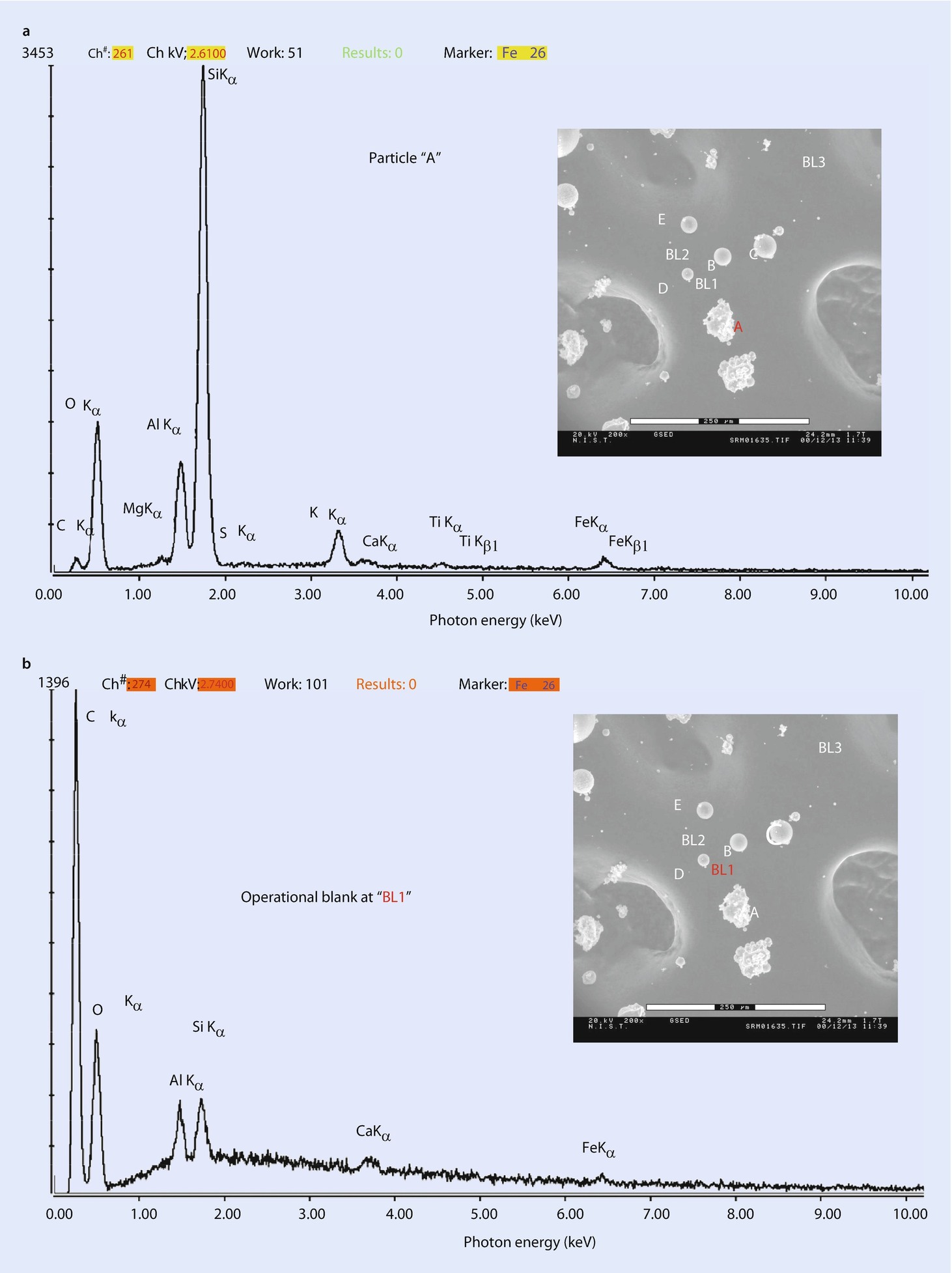
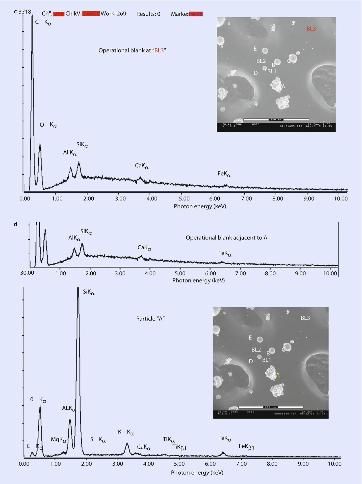
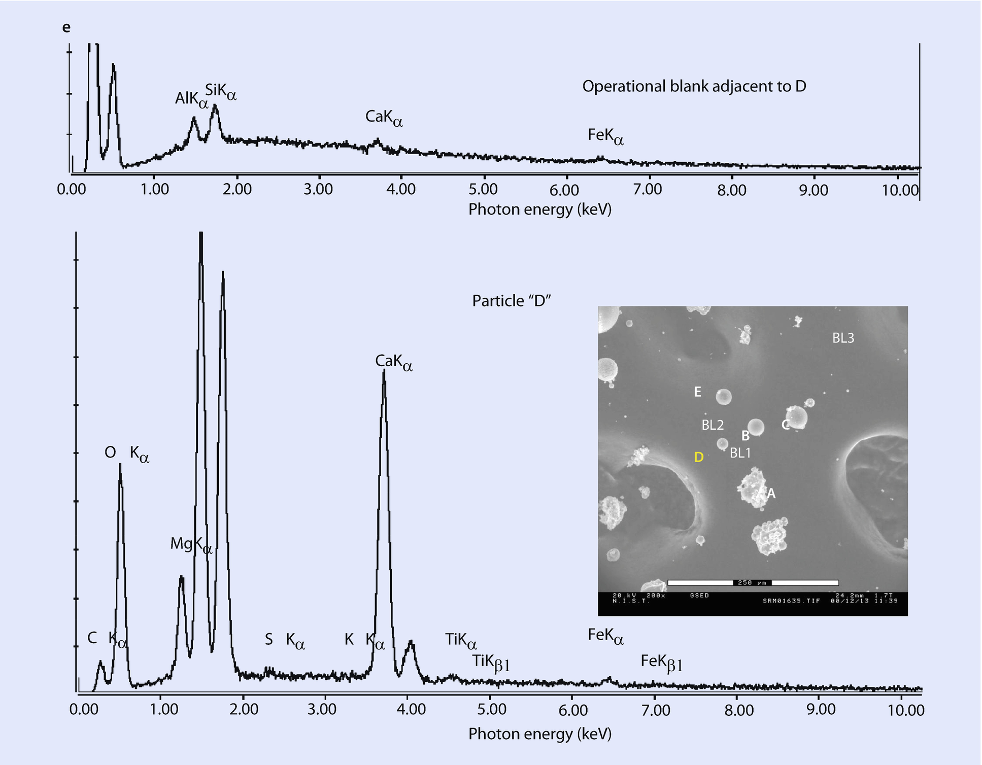
a VPSEM image of a cluster of particles and an EDS X-ray spectrum measured with the beam placed on one of them, particle “A.” b EDS X-ray spectrum measured with the beam placed on the substrate at location BL1 so that only the beam skirt excites the particles. c EDS X-ray spectrum measured with the beam placed on the substrate at location BL3 so that only the beam skirt excites the particles. d Use of analytical blank to aid interpretation of the EDS spectrum of Particle “A.” e Use of analytical blank to aid interpretation of the EDS spectrum of Particle “A”

25.2.3 Unfavorable Sample Characteristics

EDS analysis in VPSEM is most problematic for specimens consisting of densely packed microscopic features, for example, most solid materials, natural and synthetic, with a microstructure. The measured EDS X-ray spectrum in such a case depends very strongly on the VPSEM conditions, the dimensions of the target area of interest, and the exact nature of the surrounding microstructure. An example is presented in ◘ Fig. 25.14, which shows the microstructure of Raney nickel, an aluminum-nickel catalyst. Based on the contrast in this SEM-BSE image, there are three different phases present denoted D, I, and B, with different Al/Ni ratios. The spectral intensities for Al and Ni show differences in the low pressure EDS spectra shown in ◘ Fig. 25.15a that are sufficient to readily distinguish the phases despite the gas scattering (E ₀ = 20 keV; 50 Pa; water vapor; 6-mm gas path length). When the pressure is increased to 665 Pa, two of the phases can no longer be distinguished in the EDS spectrum shown in ◘ Fig. 25.15b. This loss of phase recognition is also seen as a loss of contrast in X-ray mapping, as seen in the elemental intensity maps shown in ◘ Fig. 25.16a, b.

../images/271173_4_En_25_Chapter/271173_4_En_25_Fig14_HTML.jpg — Fig. 25.14
SEM-BSE image of Raney nickel in a VPSEM

../images/271173_4_En_25_Chapter/271173_4_En_25_Fig15_HTML.png — Fig. 25.15
a EDS spectra obtained at locations “D”, “I,” and “B.” E ₀ = 20 keV; water vapor; 50 Pa, 6-mm gas path length. b EDS spectra obtained at locations “D,” “I,” and “B.” E ₀ = 20 keV; water vapor; 665 Pa, 6-mm gas path length

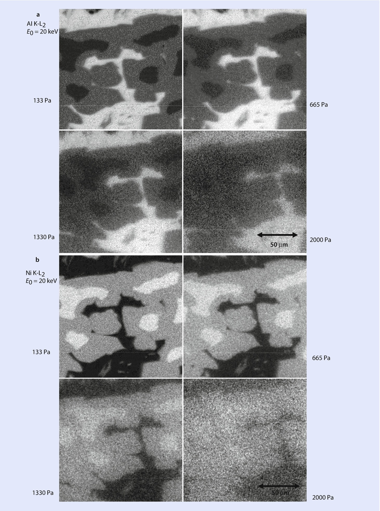
../images/271173_4_En_25_Chapter/271173_4_En_25_Fig16_HTML.jpg — Fig. 25.16
a Elemental intensity map for Al K-L₂ at various pressures (E ₀ = 20 keV, water vapor and 6-mm gas path length). b Elemental intensity map for NiKα at various pressures (E ₀ = 20 keV, water vapor and 6-mm gas path length)

Open Access This chapter is licensed under the terms of the Creative Commons Attribution-NonCommercial 2.5 International License (http://creativecommons.org/licenses/by-nc/2.5/), which permits any noncommercial use, sharing, adaptation, distribution and reproduction in any medium or format, as long as you give appropriate credit to the original author(s) and the source, provide a link to the Creative Commons license and indicate if changes were made.

The images or other third party material in this chapter are included in the chapter's Creative Commons license, unless indicated otherwise in a credit line to the material. If material is not included in the chapter's Creative Commons license and your intended use is not permitted by statutory regulation or exceeds the permitted use, you will need to obtain permission directly from the copyright holder.