Joseph I. Goldstein, Dale E. Newbury, Joseph R. Michael, Nicholas W.M. Ritchie, John Henry J. Scott and David C. JoyScanning Electron Microscopy and X-Ray Microanalysishttps://doi.org/10.1007/978-1-4939-6676-9_4
4. X-Rays
Joseph I. Goldstein1, Dale E. Newbury2, Joseph R. Michael3, Nicholas W. M. Ritchie2, John Henry J. Scott2 and David C. Joy4
(1)
University of Massachusetts, Amherst, Massachusetts, USA
(2)
National Institute of Standards and Technology, Gaithersburg, Maryland, USA
(3)
Sandia National Laboratories, Albuquerque, New Mexico, USA
(4)
University of Tennessee, Knoxville, Tennessee, USA
4.1 Overview
Energetic beam electrons stimulate the atoms of the specimen to emit “characteristic” X-ray photons with sharply defined energies that are specific to each atom species. The critical condition for generating characteristic X-rays is that the energy of the beam electron must exceed the electron binding energy, the critical ionization energy Ec, for the particular atom species and the K-, L-, M-, and/or N- atomic shell(s). For efficient excitation, the incident beam energy should be at least twice the critical excitation energy, E0 > 2 Ec. Characteristic X-rays can be used to identify and quantify the elements present within the interaction volume. Simultaneously, beam electrons generate bremsstrahlung, or braking radiation, which creates a continuous X-ray spectrum, the “X-ray continuum,” whose energies fill the range from the practical measurement threshold of 50 eV to the incident beam energy, E0. This continuous X-ray spectrum forms a spectral background beneath the characteristic X-rays which impacts accurate measurement of the characteristic X-rays and determines a finite concentration limit of detection. X-rays are generated throughout a large fraction of the electron interaction volume. The spatial resolution, lateral and in-depth, of electron-excited X-ray microanalysis can be roughly estimated with a modified Kanaya–Okayama range equation or much more completely described with Monte Carlo electron trajectory simulation. Because of their generation over a range of depth, X-rays must propagate through the specimen to reach the surface and are subject to photoelectric absorption which reduces the intensity at all photon energies, but particularly at low energies.
4.2 Characteristic X-Rays
4.2.1 Origin
The process of generating characteristic X-rays is illustrated for a carbon atom in ◘ Fig. 4.1. In the initial ground state, the carbon atom has two electrons in the K-shell bound to the nucleus of the atom with an “ionization energy” Ec (also known as the “critical excitation energy,” the “critical absorption energy,” and the “K-edge energy”) of 284 eV and four electrons in the L-shell, two each in the L1 and the L2 subshells bound to the atom, with an ionization energy of 7 eV. An incident energetic beam electron having initial kinetic energy Ein > Ec can scatter inelastically with a K-shell atomic electron and cause its ejection from the atom, providing the beam electron transfers to the atomic electron kinetic energy at least equal to the ionization energy, which is the minimum energy necessary to promote the atomic electron out of the K-shell beyond the effective influence of the positive nuclear charge. The total kinetic energy transferred to the K-shell atomic electron can range up to half the energy of the incident electron. The outgoing beam electron thus suffers energy loss corresponding to the carbon K-shell ionization energy EK = 284 eV plus whatever additional kinetic energy is imparted:
(4.1)
The ionized carbon atom is left with a vacancy in the K-shell which places it in a raised energy state that can be lowered through the transition of an electron from the L-shell to fill the K-vacancy. The difference in energy between these shells must be expressed through one of two possible routes:
1.
The left branch in ◘ Fig. 4.1 involves the transfer of this K–L inter-shell transition energy difference to another L-shell electron, which is then ejected from the atom with a specific kinetic energy:
Fig. 4.1
Schematic diagram of the process of X-ray generation: inner shell ionization by inelastic scattering of an energetic beam electron that leaves the atom in an elevated energy state which it can lower by either of two routes involving the transition of an L-shell electron to fill the K-shell vacancy: (1) the Auger process, in which the energy difference EK – EL is transferred to another L-shell electron, which is ejected with a characteristic energy: EK – EL – EL; (2) photon emission, in which the energy difference EK – EL is expressed as an X-ray photon of characteristic energy
(4.2a)
This process leaves the atom with two L-shell vacancies for subsequent vacancy-filling transitions. This ejected electron is known as an “Auger electron,” and measurement of its characteristic kinetic energy can identify the atom species of its origin, forming the physical basis for “Auger electron spectroscopy.”
2.
The right branch in ◘ Fig. 4.1 involves the creation of an X-ray photon to carry off the inter-shell transition energy:
(4.2b)
Because the energies of the atomic shells of an element are sharply defined, the shell difference is also a sharply defined quantity, so that the resulting X-ray photon has an energy that is characteristic of the particular atom species and the shells involved and is thus designated as a “characteristic X-ray.” Characteristic X-rays are emitted uniformly in all directions over the full unit sphere with 4 π steradians solid angle. Extensive tables of characteristic X-ray energies for elements with Z ≥ 4 (beryllium) are provided in the database embedded within the DTSA-II software. The characteristic X-ray photon energy has a very narrow range of just a few electronvolts depending on atomic number, as shown in ◘ Fig. 4.2 for the K–L3 transition.
Fig. 4.2
Natural width of K-shell X-ray peaks up to 25 keV photon energy (Krause and Oliver 1979)
4.2.2 Fluorescence Yield
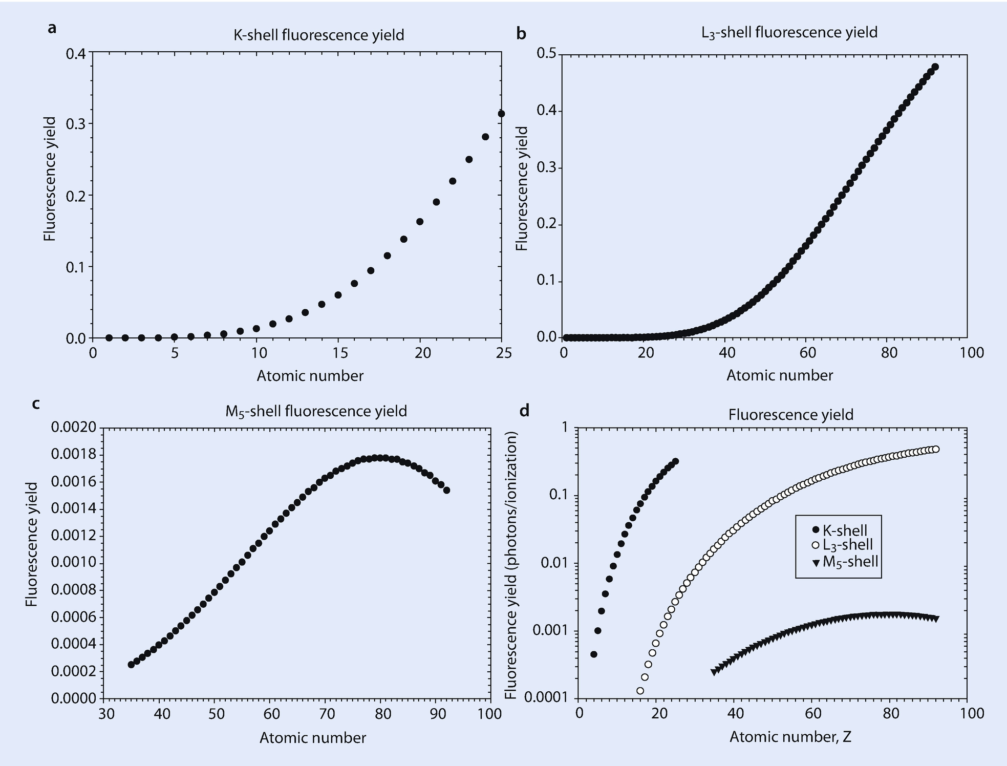
The Auger and X-ray branches in ◘ Fig. 4.1 are not equally probable. For a carbon atom, characteristic X-ray emission only occurs for approximately 0.26 % of the K-shell ionizations. The fraction of the ionizations that produce photons is known as the “fluorescence yield,” ω. Most carbon K-shell ionizations thus result in Auger electron emission. The fluorescence yield is strongly dependent on the atomic number of the atom, increasing rapidly with Z, as shown in ◘ Fig. 4.3a for K-shell ionizations. L-shell and M-shell fluorescence yields are shown in ◘ Fig. 4.3b, c; and K-, L-, and M-shell yields are compared in ◘ Fig. 4.3d (Crawford et al. 2011). From ◘ Fig. 4.3d, it can be observed that, when an element can be measured with two different shells, ωK > ωL > ωM.
Fig. 4.3
a Fluorescence yield (X-rays/ionization) from the K-shell. b Fluorescence yield (X-rays/ionization) from the L3-shell. c Fluorescence yield (X-rays/ionization) from the M5-shell. d Comparison of fluorescence yields from the K-, L3- and M5- shells (Crawford et al. 2011)
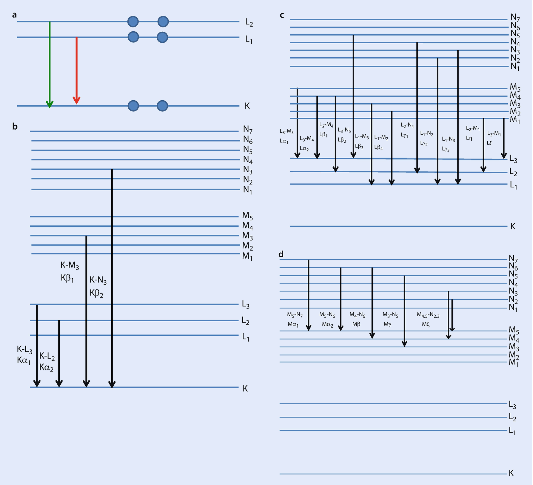
The shell transitions for carbon are illustrated in the shell energy diagram shown in ◘ Fig. 4.4a. Because of the small number of carbon atomic electrons, the shell energy values are limited, and only one characteristic X-ray energy is possible for carbon with a value of 277 eV. (The apparent possible transition from the L1-shell to the K-shell is forbidden by the quantum mechanical rules that govern these inter-shell transitions.)
Fig. 4.4
a Atomic shell energy level diagram for carbon illustrating the permitted shell transition K–L2 (shown in green) and the forbidden transition K–L1 (shown in red). b Atomic shell energy level diagram illustrating possible K-shell vacancy-filling transitions. c Atomic shell energy level diagram illustrating possible L-shell vacancy-filling transitions. d Atomic shell energy level diagram illustrating some possible M-shell vacancy-filling transitions
4.2.3 X-Ray Families
As the atomic number increases, the number of atomic electrons increases and the shell structure becomes more complex. For sodium, the outermost electron occupies the M-shell, so that a K-shell vacancy can be filled by a transition from the L-shell or the M-shell, producing two different characteristic X-rays, designated
(4.3a)
(4.3b)
For atoms with higher atomic number than sodium, additional possibilities exist for inter-shell transitions, as shown in ◘ Fig. 4.4b, leading to splitting of the K − L2,3 into K − L3 and K − L2 (Kα into Kα1 and Kα2), and similarly for Kβ into Kβ1 and Kβ2, which can be observed with energy dispersive spectrometry for X-rays with energies above 20 keV.
As these additional inter-shell transitions become possible, increasingly complex “families” of characteristic X-rays are created, as shown in the energy diagrams of ◘ Fig. 4.4c for L-shell X-rays, and 4.4d for M-shell X-rays. Only transitions that lead to X-rays that are measurable on a practical basis with energy dispersive X-ray spectrometry are shown. (There are, for example, at least 25 L-shell transitions that are possible for a heavy element such as gold, but most are of such low abundance or are so close in energy to a more abundant transition as to be undetectable by energy dispersive X-ray spectrometry.)
4.2.4 X-Ray Nomenclature
Two systems are in use for designating X-rays. The traditional but now archaic Siegbahn system lists the shell where the original ionization occurs followed by a Greek letter or other symbol that suggests the order of the family members by their relative intensity, α > β > γ > η > ζ. For closely related members, numbers are also attached, for example, Lβ1 through Lβ15. Additionally, Latin letters are used for the complex minor L-shell family members: l, s, t, u, and v. While still the predominant labeling system used in commercial X-ray microanalysis software systems, the Siegbahn system has been officially replaced by the International Union of Pure and Applied Chemistry (IUPAC) labeling protocol in which the first term denotes the shell or subshell where the original ionization occurs while the second term indicates the subshell from which the electron transition occurs to fill the vacancy; for example, Kα1 is replaced by K-L3 for a K-shell ionization filled from the L3 subshell. ◘ Table 4.1 gives the correspondence between the Siegbahn and IUPAC labeling schemes for the characteristic X-rays likely to be detected by energy dispersive X-ray spectrometry. Note that for the M-shell, there are minor family members detectable by EDS for which there are no Siegbahn designations.
Table 4.1
Correspondence between the Siegbahn and IUPAC nomenclature protocols (restricted to characteristic X-rays observed with energy dispersive X-ray spectrometry and photon energies from 100 eV to 25 keV)
Siegbahn
IUPAC
Siegbahn
IUPAC
Siegbahn
IUPAC
Kα1
K-L3
Lα1
L3-M5
Mα1
M5-N7
Kα2
K-L2
Lα2
L3-M4
Mα2
M5-N6
Kβ1
K-M3
Lβ1
L2-M4
Mβ
M4-N6
Kβ2
K-N2,3
Lβ2
L3-N5
Mγ
M3-N5
Lβ3
L1-M3
Mζ
M4,5-N2,3
Lβ4
L1-M2
M3-N1
Lγ1
L2-N4
M2-N1
Lγ2
L1-N2
M3-N4,5
Lγ3
L1-N3
M3-O1
Lγ4
L1-O4
M3-O4,5
Lη
L2-M1
M2-N4
Ll
L3-M1
4.2.5 X-Ray Weights of Lines
Within these families, the relative abundances of the characteristic X-rays are not equal. For example, for sodium the ratio of the K-L2,3 to K-M is approximately 150:1, and this ratio is a strong function of the atomic number, as shown in ◘ Fig. 4.5a for the K-shell (Heinrich et al. 1979). For the L-shell and M-shell, the X-ray families have more members, and the relative abundances are complex functions of atomic number, as shown in ◘ Fig. 4.5b, c.
Fig. 4.5
a Relative abundance of the K-L2,3 to K-M (Kα to Kβ) (Heinrich et al. 1979). b Relative abundance of the L-shell X-rays, L3-M4,5 (Lα1,2) = 1 (Crawford et al. 2011). c Relative abundance of the M-shell X-rays, M5-N6,7 (Mα) = 1 (Crawford et al. 2011)
4.2.6 Characteristic X-Ray Intensity
4.2.6.1 Isolated Atoms
When isolated atoms are considered, the probability of an energetic electron with energy E (keV) ionizing an atom by ejecting an atomic electron bound with ionization energy Ec (keV) can be expressed as a cross section, QI:
(4.4)
where ns is the number of electrons in the shell or subshell (e.g., nK = 2), and bs and cs are constants for a given shell (e.g., bK = 0.35 and cK = 1) (Powell 1976). The behavior of the ionization cross section for the silicon K-shell as a function of the energy of the energetic beam electron is shown in ◘ Fig. 4.6. Starting with a zero value at 1.838 keV, the K-shell ionization energy for silicon, the cross section rapidly increases to a peak value, and then slowly decreases with further increases in the beam energy.
Fig. 4.6
Ionization cross section for the silicon K-shell calculated with Eq. 4.4
The relationship of the energy of the exciting electron to the ionization energy of the atomic electron is an important parameter and is designated the “overvoltage,” U:
(4.5a)
The overvoltage that corresponds to the incident beam energy, E0, which is the maximum value because the beam electrons subsequently lose energy due to inelastic scattering as they progress through the specimen, is designated as U0:
(4.5b)
For ionization to occur followed by X-ray emission, U > 1. With this definition for U, Eq. (4.4) can be rewritten as
(4.6)
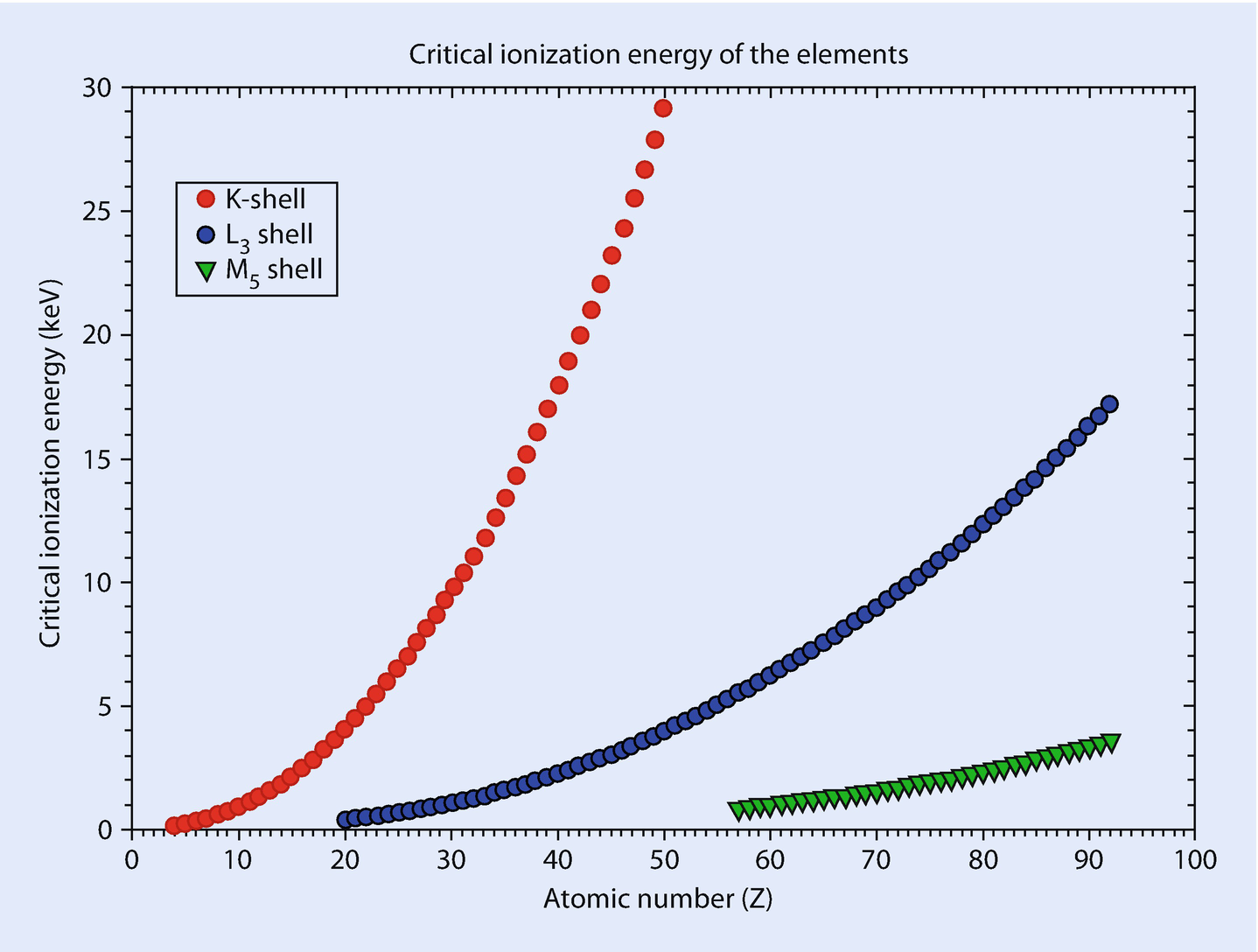
The critical excitation energy is a strong function of the atomic number of the element and of the particular shell, as shown in ◘ Fig. 4.7. Thus, for a specimen that consists of several different elements, the initial overvoltage U0 will be different for each element, which will affect the relative generation intensities of the different elements.
Fig. 4.7
Critical ionization energy for the K-, L-, and M-shells
4.2.6.2 X-Ray Production in Thin Foils
Thin foils may be defined as having a thickness such that most electrons pass through the foil without suffering elastic scattering out of the ideal beam cylinder (defined by the circular beam footprint on the entrance and exit surfaces and the foil thickness) and without suffering significant energy loss. The X-ray production in a thin foil of thickness t can be estimated from the cross section by calculating the effective density of atom targets within the foil:
(4.7)
where A is the atomic weight and N0 is Avogadro’s number.
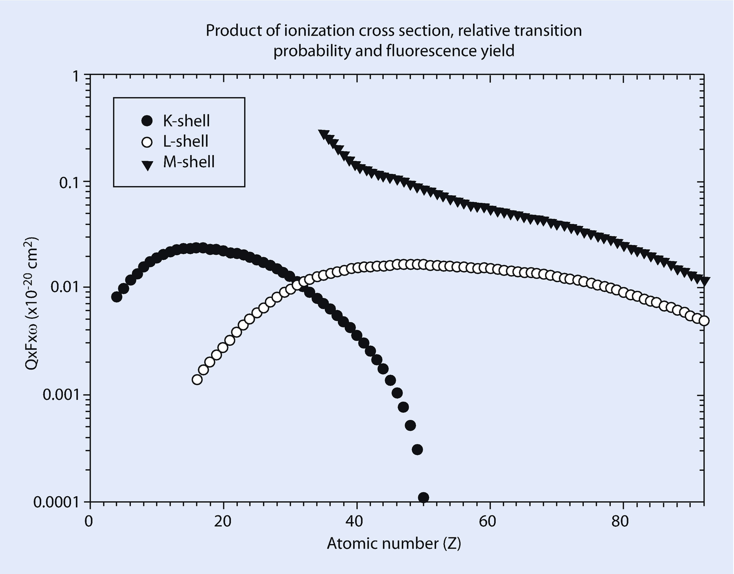
When several elements are mixed at the atomic level in a thin specimen, the relative production of X-rays from different elements depends on the cross section and fluorescence yield, as given in Eq. 4.7, and also on the partitioning of the X-ray production among the various possible members of the X-ray families, as plotted in ◘ Fig. 4.5a–c. The relative production for the most intense transition in each X-ray family is plotted in ◘ Fig. 4.8 for E0 = 30 keV. ◘ Figure 4.8 reveals strong differences in the relative abundance of the X-rays produced by different elements. This plot also reveals that over certain atomic number ranges, two different atomic shells can be excited for each element, for example, K and L for Z = 16 to Z = 50, and L and M for Z = 36 to Z = 92. For lower values of E0, these atomic number ranges will be diminished.
Fig. 4.8
Product of the ionization cross section, the fluorescence yield, and the relative weights of lines for the most intense member of the K-, L-, and M-shells for E0 = 30 keV
4.2.6.3 X-Ray Intensity Emitted from Thick, Solid Specimens
A thick specimen is one with sufficient thickness so that it contains the full electron interaction volume, which generally requires a thickness of at least a few micrometers for most choices of composition and incident beam energy. Within the interaction volume, the complete range of elastic and inelastic scattering events occur. X-ray generation for each atom species takes place across the full energy range of the ionization cross section from the initial value corresponding to the energy of the incident beam as it enters the specimen down to the ionization energy of each atom species. Based upon experimental measurements, the X-ray intensity emitted from thick targets is found to follow an expression of the form
(4.8)
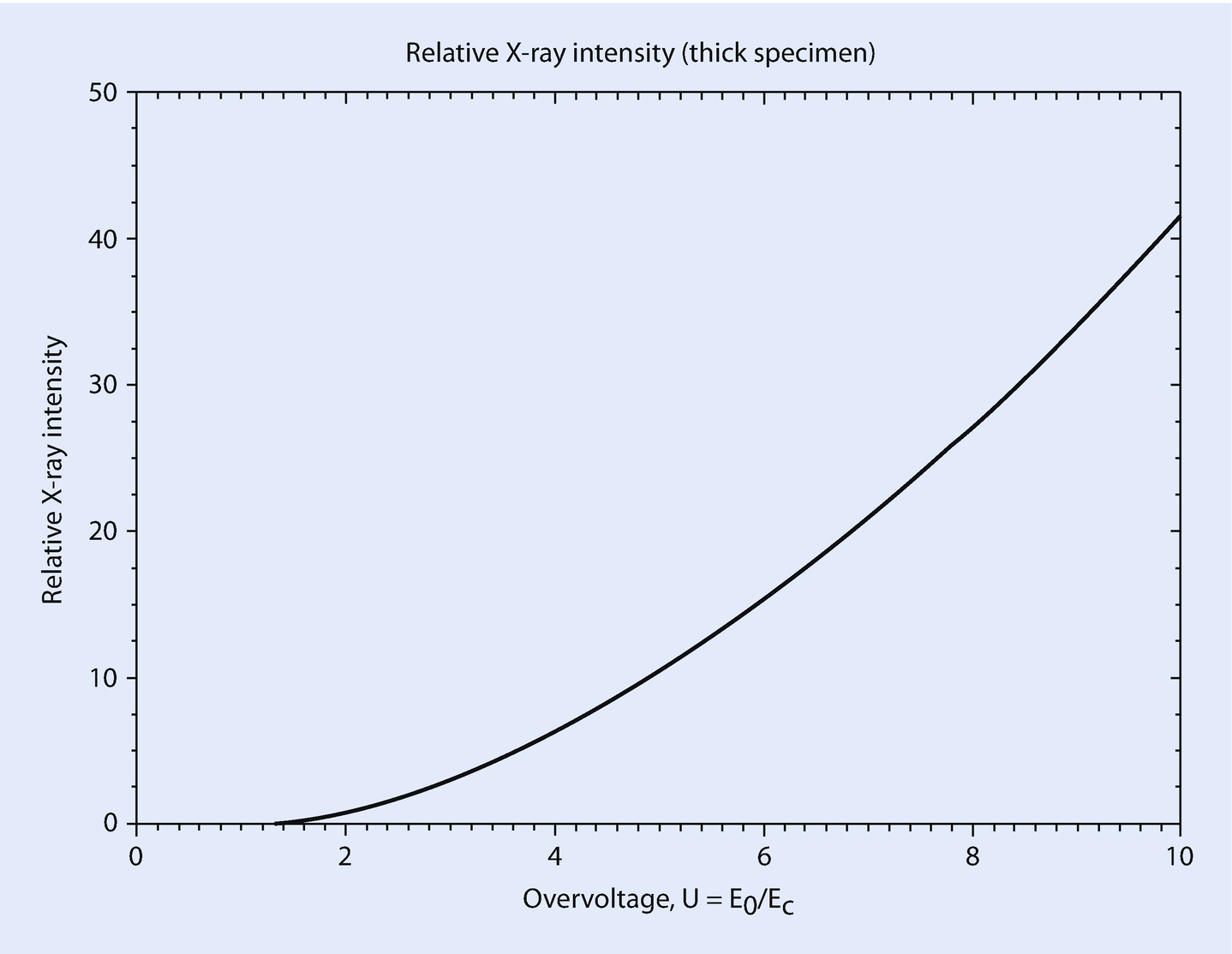
where ip is the beam current, and n is a constant depending on the particular element and shell (Lifshin et al. 1980). The value of n is typically in the range 1.5–2.0. Equation 4.8 is plotted for an exponent of n = 1.7 in ◘ Fig. 4.9. The intensity rises rapidly from a zero value at U = 1. For a reasonably efficient degree of X-ray excitation, it is desirable to select E0 so that U0 > 2 for the highest value of Ec among the elements of interest.
Fig. 4.9
Characteristic X-ray intensity emitted from a thick specimen; exponent n = 1.7
4.3 X-Ray Continuum (bremsstrahlung)
Simultaneously with the inner shell ionization events that lead to characteristic X-ray emission, a second physical process operates to generate X-rays, the “braking radiation,” or bremsstrahlung, process. As illustrated in ◘ Fig. 4.10, because of the repulsion that the beam electron experiences in the negative charge cloud of the atomic electrons, it undergoes deceleration and loses kinetic energy, which is released as a photon of electromagnetic radiation. The energy lost due to deceleration can take on any value from a slight deceleration involving the loss of a few electron volts up to the loss of the total kinetic energy carried by the beam electron in a single event. Thus, the bremsstrahlung X-rays span all energies from a practical threshold of 100 eV up to the incident beam energy, E0, which corresponds to an incident beam electron suffering total energy loss by deceleration in the Coulombic field of a surface atom as the beam electron enters the target and before it has lost any energy in any other inelastic scattering events. The braking radiation process thus forms a continuous energy spectrum, also referred to as the “X-ray continuum,” from 100 eV to E0, which is the so-called Duane–Hunt limit. The X-ray continuum forms a background beneath any characteristic X-rays produced by the atoms. The bremsstrahlung process is anisotropic, being somewhat peaked in the direction of the electron travel. In thin specimens where the beam electron trajectories are nearly aligned, this anisotropy can result in a different continuum intensity in the forward direction along the beam relative to the backward direction. However, in thick specimens, the near-randomization of the beam electron trajectory segments by elastic scattering effectively smooths out this anisotropy, so that the X-ray continuum is effectively rendered isotropic.
Fig. 4.10
Schematic illustration of the braking radiation (bremsstrahlung) process giving rise to the X-ray continuum
4.3.1 X-Ray Continuum Intensity
The intensity of the X-ray continuum, Icm, at an energy Eν is described by Kramers (1923) as
(4.9)
where ip is the incident beam current and Z is the atomic number. For a particular value of the incident energy, E0, the intensity of the continuum decreases rapidly relative to lower photon energies as Eν approaches E0, the Duane–Hunt limit.
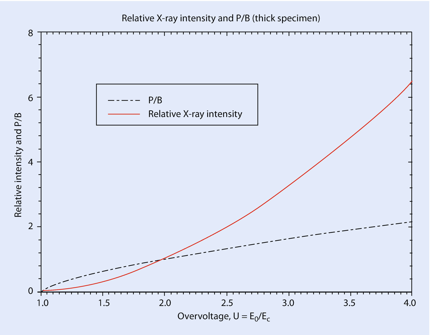
An important parameter in electron-excited X-ray microanalysis is the ratio of the characteristic X-ray intensity to the X-ray continuum intensity at the same energy, Ech = Eν, often referred to as the “peak-to-background, P/B.” The P/B can be estimated from Eqs. (4.8) and (4.9) with the approximation that Eν ≈ Ec so that Eq. (4.9) can be rewritten as—
The P/B is plotted in ◘ Fig. 4.11 with the assumption that n = 1.7, where it is seen that at low overvoltages, which are often used in electron-excited X-ray microanalysis, the characteristic intensity is low relative to higher values of U, and the intensity rises rapidly with U, while the P/B increases rapidly at low overvoltage but then more slowly as the overvoltage increases.
Fig. 4.11
X-ray intensity emitted from a thick specimen and P/B, both as a function of overvoltage with exponent n = 1.7
4.3.2 The Electron-Excited X-Ray Spectrum, As-Generated
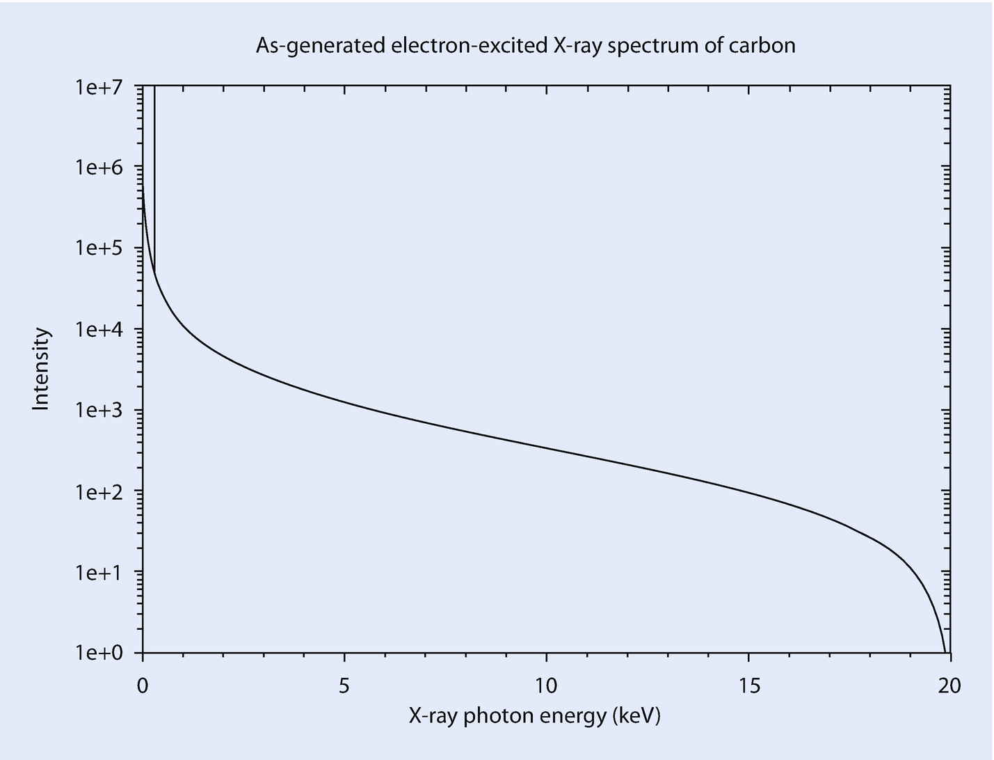
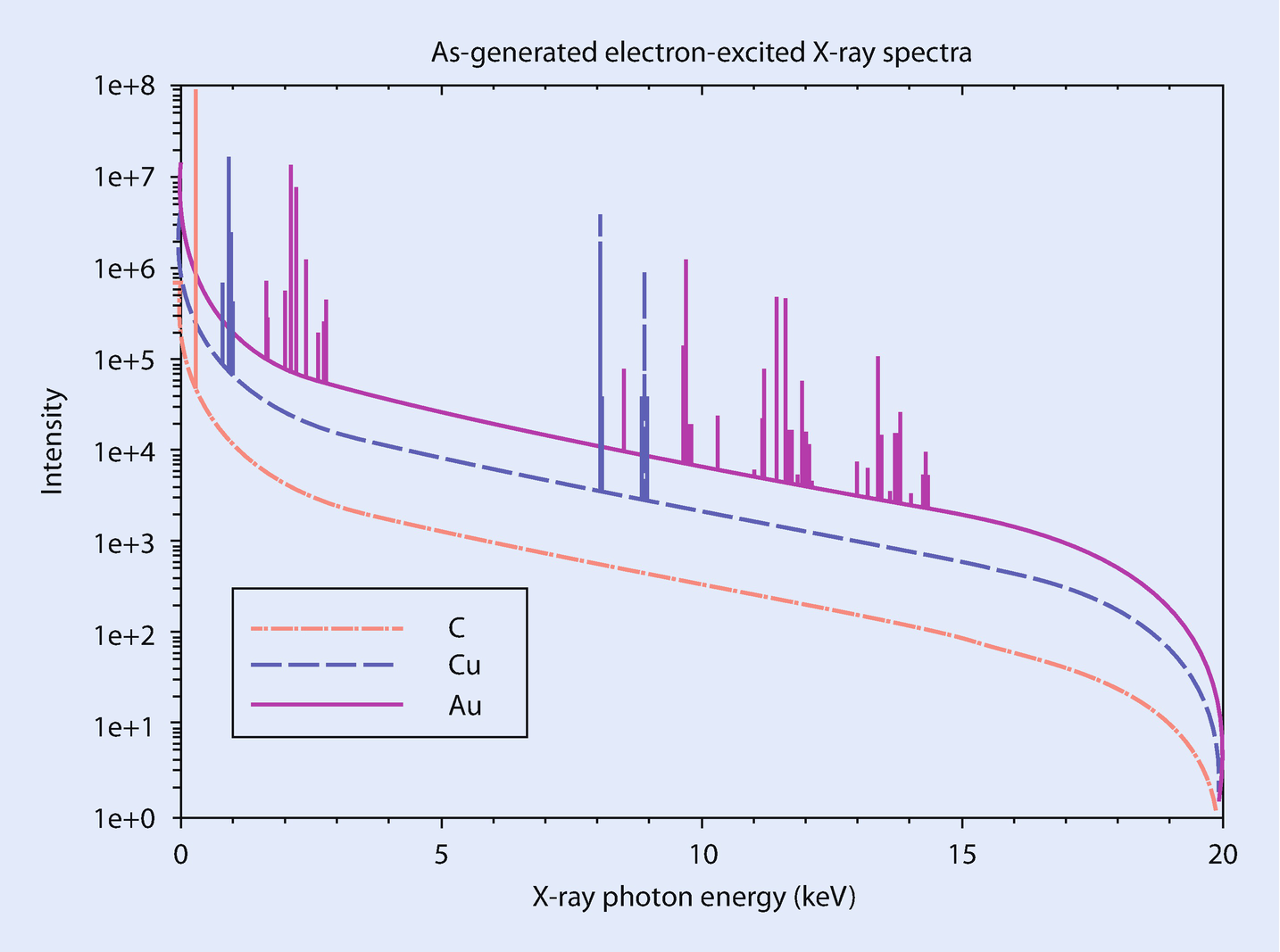
The electron-excited X-ray spectrum generated within the target thus consists of characteristic and continuum X-rays and is shown for pure carbon with E0 = 20 keV in ◘ Fig. 4.12, as calculated with the spectrum simulator in NIST Desktop Spectrum Analyzer (Fiori et al. 1992), using the Pouchou and Pichoir expression for the K-shell ionization cross section and the Kramers expression for the continuum intensity (Pouchou and Pichoir 1991; Kramers 1923). Because of the energy dependence of the continuum given by Eq. 4.10, the generated X-ray continuum has its highest intensity at the lowest photon energy and decreases at higher photon energies, reaching zero intensity at E0. By comparison, the energy span of the characteristic C–K peak is its natural width of only 1.6 eV, which is related to the lifetime of the excited K-shell vacancy. The energy width for K-shell emission up to 25 keV photon energy is shown in ◘ Fig. 4.2 (Krause and Oliver 1979). For photon energies below 25 keV, the characteristic X-ray peaks from the K-, L-, and M- shells have natural widths less than 10 eV. In the calculated spectrum of ◘ Fig. 4.12, the C–K peak is therefore plotted as a narrow line. (X-ray peaks are often referred to as “lines” in the literature, a result of their appearance in high-energy resolution measurements of X-ray spectra by diffraction-based X-ray spectrometers.) The X-ray spectra as-generated in the target for carbon, copper, and gold are compared in ◘ Fig. 4.13, where it can be seen that at all photon energies the intensity of the X-ray continuum increases with Z, as given by Eq. 4.9. The increased complexity of the characteristic X-rays at higher Z is also readily apparent.
Fig. 4.12
Spectrum of pure carbon as-generated within the target calculated for E0 = 20 keV with the spectrum simulator in Desktop Spectrum Analyzer
Fig. 4.13
Spectra of pure carbon, copper, and gold as-generated within the target calculated for E0 = 20 keV with the spectrum simulator in Desktop Spectrum Analyzer (Fiori et al. 1992)
4.3.3 Range of X-ray Production
As the beam electrons scatter inelastically within the target and lose energy, inner shell ionization events can be produced from U0 down to U = 1, so that depending on E0 and the value(s) of Ec represented by the various elements in the target, X-rays will be generated over a substantial portion of the interaction volume. The “X-ray range,” a crude estimate of the limiting range of X-ray generation, can be obtained from a simple modification of the Kanaya–Okayama range equation (IV-5) to compensate for the portion of the electron range beyond which the energy of beam electrons has deceased below a specific value of Ec:
(4.12)
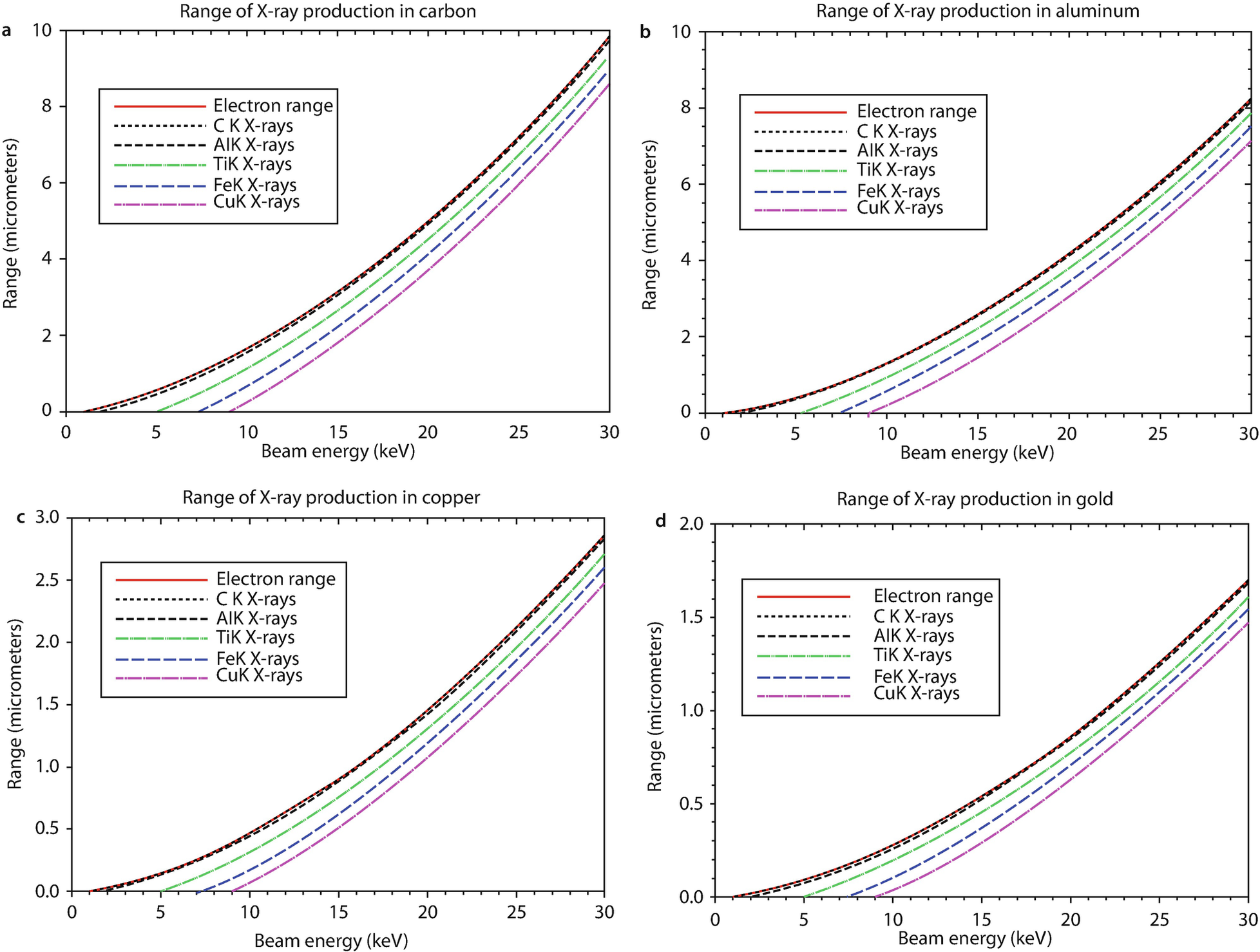
◘ Table 4.2 lists calculations of the range of generation for copper K-shell X-rays (Ec = 8.98 keV) produced in various host elements, for example, a situation in which copper is present at a low level so it has a negligible effect on the overall Kanaya–Okayama range. As the incident beam energy decreases to E0 = 10 keV, the range of production of copper K-shell X-rays decreases to a few hundred nanometers because of the very low overvoltage, U0 = 1.11. The X-ray range in various matrices for the generation of various characteristic X-rays spanning a wide range of Ec is shown in ◘ Fig. 4.14a–d.
Table 4.2
Range of Cu K-shell (Ec = 8.98 keV) X-ray generation in various matrices
Matrix
25 keV
20 keV
15 keV
10 keV
C
6.3 μm
3.9 μm
1.9 μm
270 nm
Si
5.7 μm
3.5 μm
1.7 μm
250 nm
Fe
1.9 μm
1.2 μm
570 nm
83 nm
Au
1.0 μm
630 nm
310 nm
44 nm
Fig. 4.14
a X-ray range as a function of E0 for generation of K-shell X-rays of C, Al, Ti, Fe, and Cu in a C matrix. b X-ray range as a function of E0 for generation of K-shell X-rays of C, Al, Ti, Fe, and Cu in an Al matrix. c X-ray range as a function of E0 for generation of K-shell X-rays of C, Al, Ti, Fe, and Cu in a Cu matrix. d X-ray range as a function of E0 for generation of K-shell X-rays of C, Al, Ti, Fe, and Cu in an Au matrix
4.3.4 Monte Carlo Simulation of X-Ray Generation
The X-ray range given by Eq. 4.12 provides a single value that captures the limit of the X-ray production but gives no information on the complex distribution of X-ray production within the interaction volume. Monte Carlo electron simulation can provide that level of detail (e.g., Drouin et al., 2007; Joy, 2006; Ritchie, 2015), as shown in ◘ Fig. 4.15a, where the electron trajectories and the associated emitted photons of Cu K-L3 are shown superimposed. For example, the limit of production of Cu K-L3 that occurs when energy loss causes the beam electron energy to fall below the Cu K-shell excitation energy (8.98 keV) can be seen in the electron trajectories (green) that extend beyond the region of X-ray production (red). The effects of the host element on the emission volumes for Cu K-shell and L-shell X-ray generation in three different matrices—C, Cu, and Au—is shown in ◘ Fig. 4.15a–c using DTSA-II (Ritchie 2015). The individual maps of X-ray production show the intense zone of X-ray generation starting at and continuing below the beam impact point and the extended region of gradually diminishing X-ray generation. In all three matrices, there is a large difference in the generation volume for the Cu K-shell and Cu L-shell X-rays as a result of the large difference in overvoltage at E0 = 10 keV: CuK U0 = 1.11 and CuL U0 = 10.8.
Fig. 4.15
a Monte Carlo simulation (DTSA-II) of electron trajectories and associated Cu K-shell X-ray generation in pure copper; E0 = 20 keV. b Monte Carlo simulation (DTSA-II) of the distribution of Cu K-shell and L-shell X-rays in a Cu matrix with E0 = 10 keV showing the X-rays that escape. c Monte Carlo simulation (DTSA-II) of the distribution of Cu K-shell and L-shell X-rays that escape in Au-1 % Cu with E0 = 10 keV. d Monte Carlo simulation (DTSA-II) of the distribution of Cu K-shell and L-shell X-rays that escape in C-1 % Cu with E0 = 10 keV (Ritchie 2015)
4.3.5 X-ray Depth Distribution Function, ϕ(ρz)
The distribution of characteristic X-ray production as a function of depth, designated “ϕ(ρz)” in the literature of quantitative electron-excited X-ray microanalysis, is a critical parameter that forms the basis for calculating the compositionally dependent correction (“A” factor) for the loss of X-rays due to photoelectric absorption. As shown in ◘ Fig. 4.16 for Si with E0 = 20 keV, Monte Carlo electron trajectory simulation provides a method to model ϕ(ρz) by dividing the target into layers of constant thickness parallel to the surface, counting the X-rays produced in each layer, and then plotting the intensity as a histogram. The intensity in each layer is normalized by the intensity produced in a single unsupported layer which is sufficiently thin so that no significant elastic scattering occurs: the electron trajectories pass through such a thin layer without deviation. The ϕ(ρz) distribution has several important characteristics. For a thick specimen, the intensity produced in the first layer exceeds that of the unsupported reference layer because in addition to the X-ray intensity produced by the passage of all of the beam electrons through the first layer, elastic scattering from deeper in the specimen creates backscattered electrons which pass back through the surface layer to escape the target, producing additional X-ray generation. The intensity produced in the first layer, designated ϕ0, thus always exceeds unity because of this extra X-ray production due to backscattering. Below the surface layer, ϕ(ρz) increases as elastic scattering increases the path length of the electrons that pass obliquely through each layer, compared to the relatively unscattered passage of the incident electrons through the outermost layers before elastic scattering causes significant deviation in the trajectories. The reverse passage of backscattered electrons also adds to the generation of X-rays in the shallow layers. Eventually a peak value in ϕ(ρz) is reached, beyond which the X-ray intensity decreases due to cumulative energy loss, which reduces the overvoltage, and the relative number of backscattering events decreases. The ϕ(ρz) distribution then steadily decreases to a zero intensity when the electrons have sustained sufficient energy loss to reach overvoltage U = 1. The limiting X-ray production range is given by Eq. 4.12.
Fig. 4.16
a Monte Carlo calculation of the interaction volume and X-ray production in Si with E0 = 20 keV. The histogram construction of the X-ray depth distribution ϕ(ρz) is illustrated. (Joy Monte Carlo simulation). b ϕ(ρz) distribution of generated Si K-L3 X-rays in Si with E0 = 20 keV, and the effect of absorption from each layer, giving the fraction, f(χ)depth, that escapes from each layer. The cumulative escape from all layers is f(χ) = 0.80. (Joy Monte Carlo simulation) (Joy 2006)
4.4 X-Ray Absorption
The Monte Carlo simulations shown in ◘ Fig. 4.15b–d are in fact plots of the X-rays emitted from the sample. To escape the sample, the X-rays must pass through the sample atoms where they can undergo the process of photoelectric absorption. An X-ray whose energy exceeds the binding energy (critical excitation energy) for an atomic shell can transfer its energy to the bound electron, ejecting that electron from the atom with a kinetic energy equal to the X-ray energy minus the binding energy, as shown in ◘ Fig. 4.17, which initiates the same processes of X-ray and Auger electron emission as shown in ◘ Fig. 4.1 for inner shell ionization by energetic electrons. The major difference in the two processes is that the X-ray is annihilated in photoelectric absorption and its entire energy transferred to the ejected electron. Photoelectric absorption is quantified by the “mass absorption coefficient,” μ/ρ, which determines the fraction of X-rays that pass through a thickness s of a material acting as the absorber:
Fig. 4.17
Schematic diagram of the process of X-ray generation: inner shell ionization by photoabsorption of an energetic X-ray that leaves the atom in an elevated energy state which it can lower by either of two routes involving the transition of an L-shell electron to fill the K-shell vacancy: 1 the Auger process, in which the energy difference EK – EL is transferred to another L-shell electron, which is ejected with a characteristic energy: EK – EL – EL; (2) photon emission, in which the energy difference EK – EL is expressed as an X-ray photon of characteristic energy
(4.13)
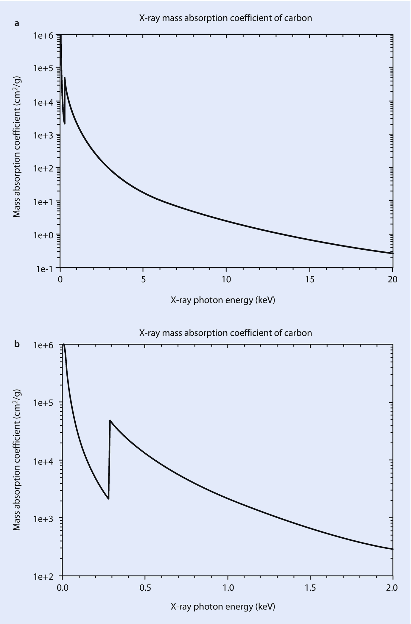
where I0 is the initial X-ray intensity and I is the intensity after passing through a thickness, s, of a material with density ρ. The dimensions of the mass absorption coefficient are cm2/g. For a given material, mass absorption coefficients generally decrease with increasing photon energy, as shown for carbon in ◘ Fig. 4.18a. The exception is near the critical excitation energy for the atomic shells of a material. The region near the C K-shell excitation energy of 284 eV is shown expanded in ◘ Fig. 4.18b, where an abrupt increase in μ/ρ occurs. An X-ray photon whose energy is just slightly greater than the critical excitation energy for an atomic shell can very efficiently couple its energy to the bound electron, resulting in a high value of μ/ρ. With further increases in photon energy, the efficiency of the coupling of the photon energy to the bound electron decreases so that μ/ρ also decreases. For more complex atoms with more atomic shells, the mass absorption coefficient behavior with photon energy becomes more complicated, as shown for Cu in ◘ Fig. 4.19a, b, which shows the region of the three Cu L-edges. For Au, ◘ Fig. 4.20a–c shows the regions of the three Au L-edges and the five Au M-edges.
Fig. 4.18
a Mass absorption coefficient for C as a function of photon energy. b Mass absorption coefficient for C as a function of photon energy near the C critical excitation energy
Fig. 4.19
a Mass absorption coefficient for Cu as a function of photon energy. b Mass absorption coefficient for Cu as a function of photon energy near the Cu L-shell critical excitation energies
Fig. 4.20
a Mass absorption coefficient for Au as a function of photon energy. b Mass absorption coefficient for Au as a function of photon energy near the Au L-shell critical excitation energies. c Mass absorption coefficient for Au as a function of photon energy near the Au M-shell critical excitation energies
When a material consists of an atomic-scale mixture of two or more elements, the mass absorption for the mixture is calculated as
(4.14)
where (μ/ρ)ij is the mass absorption coefficient for the X-rays of element i by element j, and Cj is the mass concentration of element j in the mixture.
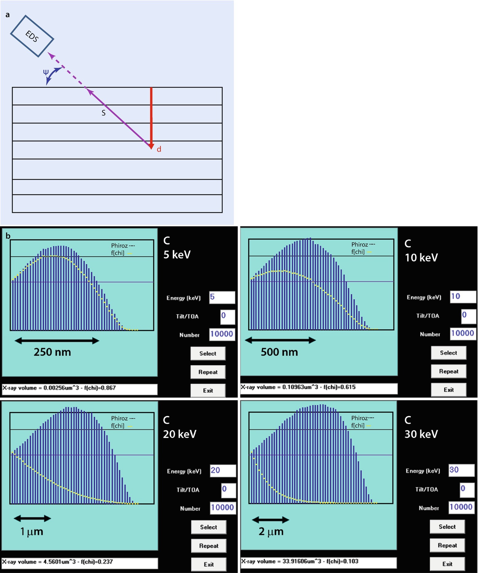
Photoelectric absorption reduces the X-ray intensity that is emitted from the target at all photon energies. The absorption loss from each layer of the ϕ(ρz) distribution is calculated using Eq. 4.15 with the absorption path, s, determined as shown in ◘ Fig. 4.21a from the depth, d, of the histogram slice, and the cosecant of the X-ray detector “take-off angle,” ψ, which is the elevation angle of the detector above the target surface:
Fig. 4.21
a Determination of the absorption path length from a layer of the ϕ(ρz) distribution located at depth, d, in the direction of the X-ray detector. b Monte Carlo determination of the ϕ(ρz) distribution and absorption for carbon at various beam energies. (Joy Monte Carlo simulation)
(4.15)
Normalizing by the intensity generated in each layer, the ϕ(ρz) histogram gives the probability, with a value between 0 and 1, that a photon generated in that layer and emitted into the solid angle of the EDS detector will escape and reach the detector, as shown in ◘ Fig. 4.16b for each histogram bin of the silicon ϕ(ρz) distribution. The escape probability of X-rays integrated over the complete ϕ(ρz) histogram gives the parameter designated “f(χ),” which is the overall escape probability, between 0 and 1, for an X-ray generated anywhere in the ϕ(ρz) distribution.
◘ Figure 4.21b shows a sequence of calculations of the C K ϕ(ρz) distribution and subsequent absorption as a function of incident beam energy. As the incident beam energy increases, the depth of electron penetration increases so that carbon characteristic X-rays are produced deeper in the target. For pure carbon with E0 = 5 keV, the cumulative value of f(χ) = 0.867; that is, 86.7 % of all carbon X-rays that are generated escape, while 13.3 % are absorbed. As the C X-rays are produced deeper with increasing beam energy, the total X-ray absorption increases so that the value of f(χ) for C K decreases sharply with increasing beam energy, as shown in ◘ Fig. 4.21b and in ◘ Table 4.3.
Table 4.3
Self-absorption of carbon K-shell X-rays as a function of beam energy
E0
f(χ)
2 keV
0.974
5
0.867
10
0.615
20
0.237
30
0.103
Thus, with E0 = 2 keV, 97.4 % of the carbon X-rays escape the specimen, while at E0 = 30 keV, nearly 90 % of the carbon X-rays generated in pure carbon are absorbed before they can exit the specimen.
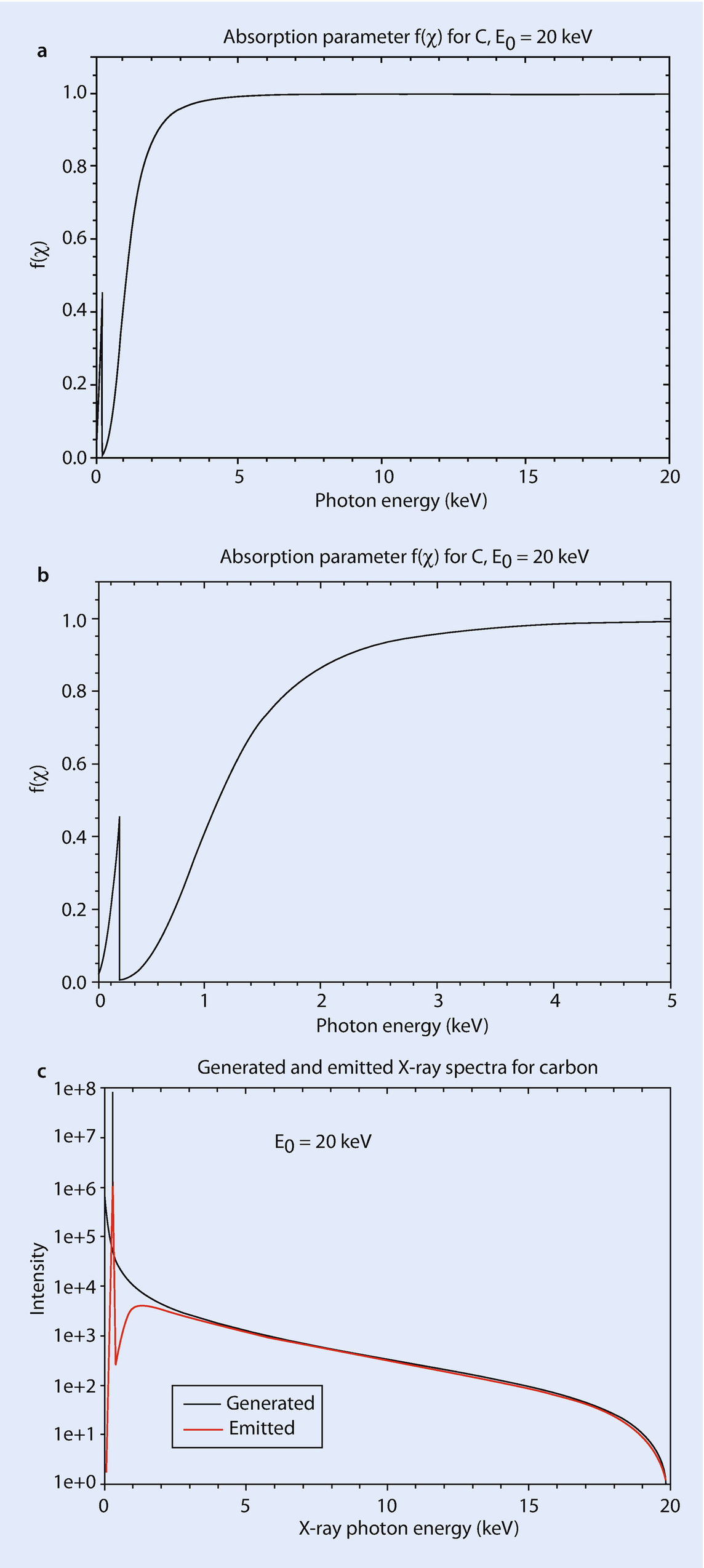
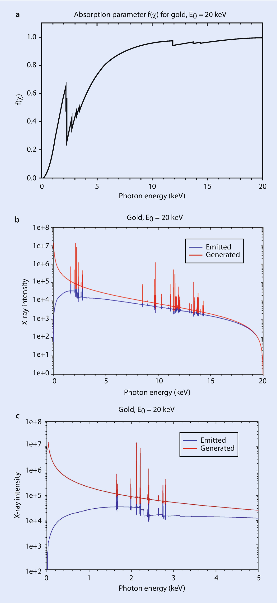
When the parameter f(χ) is plotted at every photon energy from the threshold of 100 eV up to the Duane–Hunt limit of the incident beam energy E0, X-ray absorption is seen to sharply modify the X-ray spectrum that is emitted from the target, as illustrated for carbon (◘ Fig. 4.22), copper (◘ Fig. 4.23), and gold (◘ Fig. 4.24). The high relative intensity of the X-ray continuum at low photon energies compared to higher photon energies in the generated spectrum is greatly diminished in the emitted spectrum because of the higher absorption suffered by low energy photons. Discontinuities in f(χ) are seen at the critical ionization energy of the K-shell in carbon, the K- and L-shells in copper, and the M- and L-shells in gold, corresponding to the sharp increase in μ/ρ just above the critical ionization energy. Because the X-ray continuum is generated at all photon energies, the continuum is affected by every ionization edge represented by the atomic species present, resulting in abrupt steps in the background. An abrupt decrease in X-ray continuum intensity is observed just above the absorption edge energy due to the increase in the mass absorption coefficient. The characteristic peaks in these spectra are also diminished by absorption, but because a characteristic X-ray is always lower in energy than the ionization edge energy from which it originated, the mass absorption coefficient for characteristic X-rays is lower than that for photons with energies just above the shell ionization energies. Thus an element is relatively transparent to its own characteristic X-rays because of the decrease in X-ray absorption below the ionization edge energy.
Fig. 4.22
a Absorption parameter f(χ) as a function of photon energy for carbon and an incident beam energy of E0 = 20 keV. Note the abrupt decrease for photons just above the ionization energy of carbon at 0.284 keV. b Expansion of the region from 0 to 5 keV. Note the abrupt decrease for photons just above the ionization energy of carbon at 0.284 keV. c Comparison of the generated (black) and emitted (red) X-ray spectra for carbon with an incident beam energy of E0 = 20 keV
Fig. 4.23
a Absorption parameter f(χ) as a function of photon energy for copper and an incident beam energy of E0 = 20 keV. Note the abrupt decrease just above the ionization energies of the three L-shells near 0.930 keV and the K-shell ionization energy at 8.98 keV. b Comparison of the generated (red) and emitted (blue) X-ray spectra for copper with an incident beam energy of E0 = 20 keV. c Comparison of the generated and emitted X-ray spectra for copper with an incident beam energy of E0 = 20 keV; expanded to show the region of the Cu L-shell and Cu K-shell ionization energies
Fig. 4.24
a Absorption parameter f(χ) as a function of photon energy for gold and an incident beam energy of E0 = 20 keV. Note the abrupt decrease in f(χ) for photons just above the ionization energies of the gold M-shell and gold L-shell. b Comparison of the generated (red) and emitted (blue) X-ray spectra for gold with an incident beam energy of E0 = 20 keV. c Comparison of the generated (red) and emitted (blue) X-ray spectra for gold with an incident beam energy of E0 = 20 keV; expansion of the region around the gold M-shell ionization edges
4.5 X-Ray Fluorescence
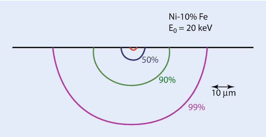
As a consequence of photoelectric absorption shown in ◘ Fig. 4.17, the atom will subsequently undergo de-excitation following the same paths as is the case for electron ionization in ◘ Fig. 4.1. Thus, the primary X-ray spectrum of characteristic and continuum X-rays generated by the beam electron inelastic scattering events gives rise to a secondary X-ray spectrum of characteristic X-rays generated as a result of target atoms absorbing those characteristic and continuum X-rays and emitting lower energy characteristic X-rays. Because continuum X-rays are produced up to E0, the Duane–Hunt limit, all atomic shells present with Ec < E0 will be involved in generating secondary X-rays, which is referred to as “secondary X-ray fluorescence” by the X-ray microanalysis community. Generally, at any characteristic photon energy the contribution of secondary fluorescence is only a few percent or less of the intensity produced by the direct electron ionization events. However, there is a substantial difference in the spatial distribution of the primary and secondary X-rays. The primary X-rays must be produced within the interaction volume of the beam electrons, which generally has limiting dimensions of a few micrometers at most. The secondary X-rays can be produced over a much larger volume because the range of X-rays in a material is typically an order-of-magnitude (or more) greater than the range of an electron beam with E0 from 5 to 30 keV. This effect is shown in ◘ Fig. 4.25 for an alloy of Ni-10 % Fe for the secondary fluorescence of Fe K-shell X-rays (EK = 7.07 keV) by the electron-excited Ni K-L2,3 X-rays (7.47 keV). The hemispherical volume that contains 99 % of the secondary Fe K-L2,3 X-rays has a radius of 30 μm.
Fig. 4.25
Range of secondary fluorescence of Fe K-L3 (EK = 7.07 keV) by Ni K-L3 X-rays (7.47 keV). Red arc = extent of direct electron excitation of Ni K-L3 and Fe K-L3. Blue arc = range for 50 % of total secondary fluorescence of Fe K-L3 by Ni K-L3; green arc = 90 %; magenta arc = 99 %
Open Access This chapter is licensed under the terms of the Creative Commons Attribution-NonCommercial 2.5 International License (http://creativecommons.org/licenses/by-nc/2.5/), which permits any noncommercial use, sharing, adaptation, distribution and reproduction in any medium or format, as long as you give appropriate credit to the original author(s) and the source, provide a link to the Creative Commons license and indicate if changes were made.
The images or other third party material in this chapter are included in the chapter's Creative Commons license, unless indicated otherwise in a credit line to the material. If material is not included in the chapter's Creative Commons license and your intended use is not permitted by statutory regulation or exceeds the permitted use, you will need to obtain permission directly from the copyright holder.

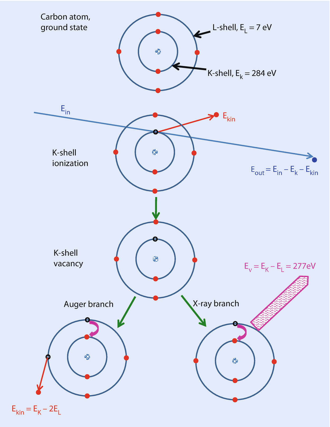 Fig. 4.1
 (4.2a)
 (4.2b)


![$$ {\displaystyle \begin{array}{l}{Q}_I\left( ionizations/\left[{e}^{-}\left( atom/c{m}^2\right)\right]\right)\ \\ {}=6.51\times {10}^{-20}\left[\left({n}_s{b}_s\right)/E\ {E}_c\right]\ lo{g}_e\left({c}_sE/{E}_c\right)\end{array}} $$](../images/271173_4_En_4_Chapter/271173_4_En_4_Chapter_TeX_Equ6.png)


![$$ {\displaystyle \begin{array}{l}{Q}_I\left( ionizations/\left[{e}^{-}\left( atom/c{m}^2\right)\right]\right)\ \\ {}=6.51\times 1{0}^{-20}\left[\left({n}_s{b}_s\right)/U\ {E_c}^2\right]\ lo{g}_e\left({c}_sU\right)\end{array}} $$](../images/271173_4_En_4_Chapter/271173_4_En_4_Chapter_TeX_Equ9.png)
![$$ {\displaystyle \begin{array}{l}{n}_X\left[ photons/{e}^{-}\right]={Q}_I\kern0.50em \left[ ionizations/{e}^{-}\left( atom/c{m}^2\right)\right]\\ {}\times \omega \left[X-\mathrm{rays}/ ionization\right]\times {N}_0\left[ atoms/ mole\right]\\ {}\times \left(1/A\right)\ \left[ moles/g\right]\times \rho \left[g/c{m}^3\right]\\ {}\times t\ \left[ cm\right]={Q}_I\times \omega \times {N}_0\times \rho \times t/A\end{array}} $$](../images/271173_4_En_4_Chapter/271173_4_En_4_Chapter_TeX_Equ10.png)
![$$ I\approx {i}_p{\left[\left({E}_0-{E}_c\right)/{E}_0\right]}^n\approx {i}_p{\left[U-1\right]}^n $$](../images/271173_4_En_4_Chapter/271173_4_En_4_Chapter_TeX_Equ11.png)

![$$ {I}_{cm}\approx {i}_pZ\ \left[\left({E}_0-{E}_{\nu}\right)/{E}_{\nu}\right] $$](../images/271173_4_En_4_Chapter/271173_4_En_4_Chapter_TeX_Equ12.png)
![$$ {I}_{cm}\approx {i}_pZ\ \left[\left({E}_0-{E}_c\right)/{E}_{\mathrm{c}}\right]\approx {i}_pZ\ \left(U-1\right) $$](../images/271173_4_En_4_Chapter/271173_4_En_4_Chapter_TeX_Equ13.png)

![$$ {R}_{K-O}(nm)=27.6\ \left(A/{Z}^{0.89}\rho \right)\ \left[{E_0}^{1.67}-{E_{\mathrm{c}}}^{1.67}\right] $$](../images/271173_4_En_4_Chapter/271173_4_En_4_Chapter_TeX_Equ15.png)


![$$ I/{I}_0=\mathit{\exp}\ \left[-\left(\mu /\rho \right)\ \rho s\right] $$](../images/271173_4_En_4_Chapter/271173_4_En_4_Chapter_TeX_Equ16.png)