Image Formation

6.1 Image Construction by Scanning Action

After leaving the electron source, the beam follows the central (optic) axis of the lens system and is sequentially defined by apertures and focused by the magnetic and/or electrostatic fields of the lens system. Within the final (objective) lens, a system of scan coils acts to displace the beam off the optic axis so that it can be addressed to a location on the specimen, as illustrated schematically for single deflection scanning in ◘ Fig. 6.1. At any particular time, there is only one ray path (solid line) through the scanning system and the beam reaches only one location on the specimen, for example, position 3 in ◘ Fig. 6.1. The SEM image is a geometric construction created under computer control by addressing the focused beam to a sequence of discrete x-y locations on the specimen and measuring the effect of the interaction of the beam with the specimen at each location. For a single gray-scale SEM image, this interaction could be the output from a single electron detector, such as the Everhart–Thornley detector. It is also possible to measure the output from more than one detector simultaneously while the beam is addressed to a single x-y location. When this is done, multiple gray-scale SEM images are built up at the same time during the scan. It is essential to realize that even when these multiple signals are being collected simultaneously and multiple images are produced, only a single scan is needed; the parallel nature of the acquisition arises from parallel detection, not parallel scanning. Note that no “true image” actually exists within the SEM in the same sense as the image created in a light optical microscope, where actual ray paths extend from each point on the specimen through the lens system to a corresponding point on the image recording medium, whether that is the eye of a human viewer or the positionally sensitive detector of a digital camera. In the SEM, at each location sampled by the incident electron beam, each signal is measured with an appropriate detector and the analog measurement is converted to an equivalent digital value (using an analog-to-digital converter, ADC). The beam x-y location and the intensity(ies) I _j of the signal(s) of interest generate a digital stream of data packets (x, y, I _j), where the index j represents the various signals available: backscattered electrons (BSE), secondary electrons (SE), absorbed current, X-rays, cathodoluminescence, etc.

../images/271173_4_En_6_Chapter/271173_4_En_6_Fig1_HTML.png — Fig. 6.1
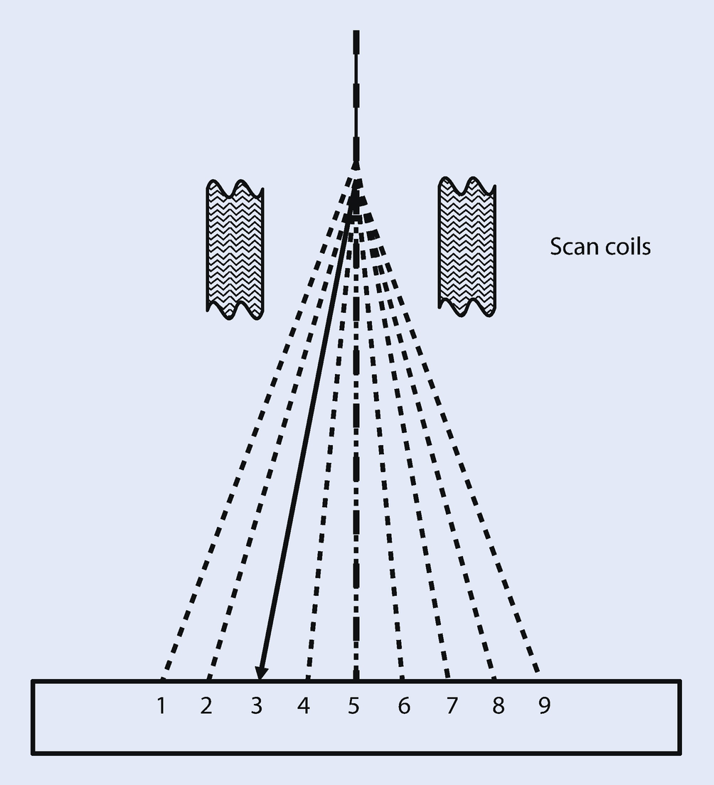
Scanning action to produce a sequence of discrete beam locations on the specimen

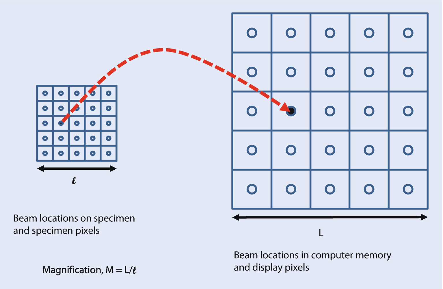
A simple description of this “scanning action” to create an image is shown schematically in ◘ Fig. 6.2, where an area with equal edge dimensions l being scanned on the specimen is effectively divided into an x-y grid of square picture elements or “pixels” of number n along an edge. The specimen pixel edge dimension is given by

../images/271173_4_En_6_Chapter/271173_4_En_6_Fig2_HTML.png — Fig. 6.2
Scanning action in two dimensions to produce an x-y raster, and the corresponding storage and display of image information by scan location

$\mathrm{Specimen}\ \mathrm{pixel}\ \mathrm{dimension}=l/n$

(6.1)

With equal values of the scan l along the x- and y-dimensions, the pixels will be square. Strictly, the pixel is the geometric center of the area defined by the edges given by Eq. (6.1), and the center-to-center spacing or pitch is given by Eq. (6.1). In creating an SEM image, the center of the beam is placed in the center of a specific pixel, dwells for a specific time, t _p, and the signal information I _sig from various sources “j”—e.g., SE, BSE, X-ray, etc.—collected during that time at that (x, y) location is stored at a corresponding location in a data matrix with a minimum of three dimensions (x, y, I _j). The final image viewed by the microscopist is created by reading the stored data matrix into a corresponding pattern of (x, y) display pixels with a total edge dimension L, and adjusting the display brightness (“gray level”, varying from black to white) according to the relative strength of the measured signal(s).

6.2 Magnification

“Magnification” in such a scanning system is given by the ratio of the edge dimensions of the specimen area and the display area:

$\mathrm{M}=\mathrm{L}/l$

(6.2)

Since the final display size is typically fixed, increasing the magnification in this scanning system means that the edge dimension of the area scanned on the specimen is reduced.

6.2.1 Magnification, Image Dimensions, and Scale Bars

One of the most important pieces of information that the microscopist seeks is the size of objects of interest. The first step in determining the size of an object is knowledge of the parameters in Eq. (6.2): the linear edge length of the area scanned on the specimen and on the display. The nominal SEM magnification appropriate to the display as viewed by the microscopist is typically embedded in the alphanumeric record that appears with the image as presented on most SEMs, as shown in the example of ◘ Fig. 6.3, and as recorded with the metadata associated with the digital record of the image. “Magnification” only has a useful meaning for the display on which the original image was viewed, since this is the display for which L in Eq. (6.2) is strictly valid. If the image is transferred to another display with a different value of L, for example, projected on a large screen, then the specific magnification value embedded in the metadata bar becomes meaningless. Much more meaningful are the x- and y-image dimensions, which are the lengths of the orthogonal boundaries of the scanned square area on the specimen, l, in ◘ Fig. 6.2, or for rectangular images, the dimensions in orthogonal directions, l by k (dimensions: millimeters, micrometers, or nanometers, as appropriate). While the image dimension(s) is a much more robust term that automatically scales with the presentation of the image, this term is also vulnerable to inadvertent mistakes, such as might happen if the image is “cropped,” either digitally or manually in hard copy and the appropriate reduction in size is not recorded by modifying l (and k, if rectangular) appropriately. The most robust measure in terms of image integrity is the dimensional scale bar, which shows the length that corresponds to a specific millimeter, micrometer, or nanometer measure. Because this feature is embedded directly in the image (as well as in the metadata associated with the image), it cannot be lost unless the image is severely (and obviously) cropped. Such a scale bar automatically enlarges or contracts as the image size is modified for subsequent publication or projection.

../images/271173_4_En_6_Chapter/271173_4_En_6_Fig3_HTML.jpg — Fig. 6.3
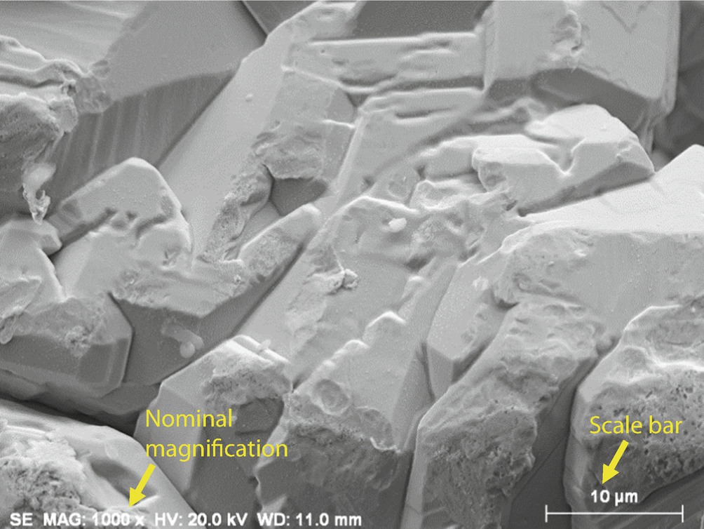
SEM-SE image of silver crystals showing a typical information bar specifying the electron detector, the nominal magnification, the accelerating voltage, and a scale bar

6.3 Making Dimensional Measurements With the SEM: How Big Is That Feature?

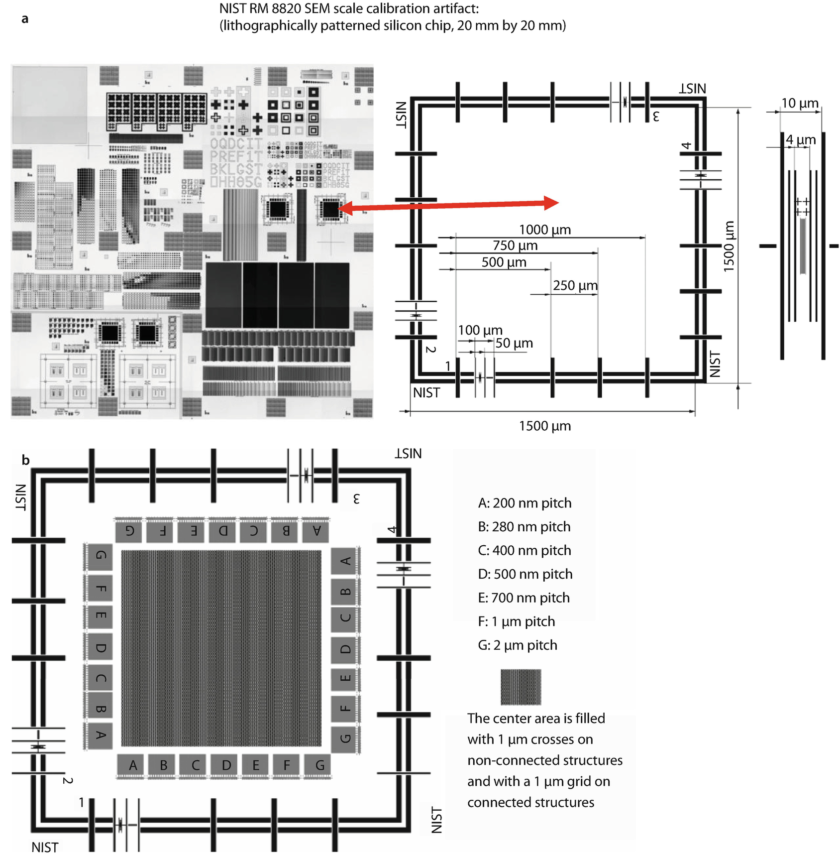
6.3.1 Calibrating the Image

The validity of the dimensional marker displayed on the SEM image should not be automatically assumed (Postek et al. 2014). As part of a laboratory quality-assurance program, the dimensional marker and/or the x- and y-dimensions of the scanned field should be calibrated and the calibration periodically confirmed. This can be accomplished with a “scale calibration artifact,” a specimen that contains features with various defined spacings whose dimensions are traceable to the fundamental primary length standard through a national measurement institution. An example of such a scale calibration artifact suitable for SEM is Reference Material RM 8820 (Postek et al. 2014; National Institute of Standards and Technology [USA]), shown in ◘ Fig. 6.4. This scale calibration artifact consists of an elaborate collection of linear features produced by lithography on a silicon substrate. It is important to calibrate the SEM over the full range of magnifications to be used for subsequent work. RM 8820 contains large-scale structures suitable for low and intermediate magnifications, for example, a span of 1500 μm (1.5 mm) as indicated by the red arrows in ◘ Fig. 6.4a, that permit calibration of scan fields ranging up to 1 × 1 cm (e.g., a nominal magnification of 10× on a 10 x 10-cm display). Scanned fields as small as 1 × 1 μm (e.g., a nominal magnification of 100,000×) can be calibrated with the series of structures with pitches of various repeat distances shown in ◘ Fig. 6.4b. The structures present in RM 8820 enable simultaneous calibration along the x- and y-axes of the image so that image distortion can be minimized. Accurate calibration in orthogonal directions is critical for establishing “square pixels” in order to avoid introducing serious distortions into the scanned image. With square pixels, the shape of an object is faithfully transferred, as shown in ◘ Fig. 6.5a, while non-square pixels in the specimen scan result in distortion in the displayed image, ◘ Fig. 6.5b.

../images/271173_4_En_6_Chapter/271173_4_En_6_Fig4_HTML.png — Fig. 6.4
a Scale calibration artifact Reference Material 8820 (National Institute of Standards and Technology, U.S.) (From Postek et al. 2014). b Detail within the feature noted in ◘ Fig. 6.4a (From Postek et al. 2014)

../images/271173_4_En_6_Chapter/271173_4_En_6_Fig5_HTML.png — Fig. 6.5
a Careful calibration of the x- and y-scans produces square pixels, and a faithful reproduction of shapes lying in the scan plane perpendicular to the optic axis. b Distortion in the display of an object caused by non-square pixels in the image scan

Note that for all measurements the calibration artifact must be placed normal to the optic axis of the SEM to eliminate image foreshortening effects (see further discussion below).

6.3.1.1 Using a Calibrated Structure in ImageJ-Fiji

The image-processing software engine ImageJ-Fiji includes a “Set Scale” function that enables a user to transfer the image calibration to subsequent measurements made with various functions. As shown in ◘ Fig. 6.6a, starting with an image of a primary or secondary calibration artifact (i.e., where “secondary” refers to a commercial vendor artifact that is traceable to a primary national measurement calibration artifact) that contains a set of defined distances, the user can specify a vector that spans a particular pitch to establish the calibration at that magnification setting. This calibration procedure should then be repeated to cover the range of magnification settings to be used for subsequent measurements of unknowns. Note that the calibration that has been performed is only strictly valid for the SEM working distance at which the calibration artifact has been imaged. When a different working distance (i.e., objective lens strength) is used subsequently to image the unknown specimen, the SEM software is likely to make automatic adjustments for different lens strength and scan dimensions that alter the effective magnification. For the most robust measurement environment, the user should use the calibration artifact to determine the validity of the SEM software specified scale at other working distances to develop a comprehensive calibration.

../images/271173_4_En_6_Chapter/271173_4_En_6_Fig6_HTML.jpg — Fig. 6.6
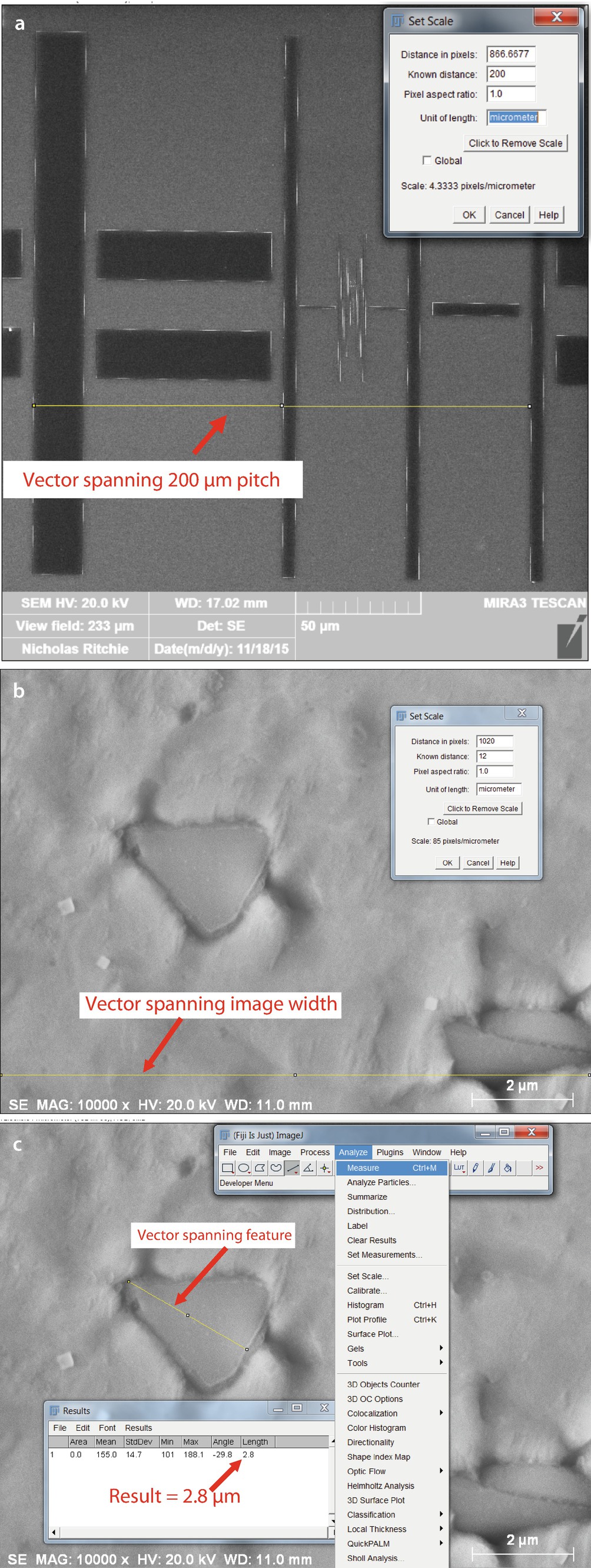
a ImageJ (Fiji) “Set Scale” calibration function applied to an image of NIST RM 8820. b ImageJ (Fiji) “Set Scale” calibration function applied to an image of an unknown (alloy IN100). c After “Set Scale” image calibration, subsequent use of ImageJ (Fiji) “Measure” function to determine the size of a feature of interest

Alternatively, if the SEM magnification calibration has already been performed with an appropriate calibration artifact, then subsequent images of unknowns will be recorded with accurate dimensional information in the form of a scale bar and/or specified scan field dimensions. This information can be used with the “Set Scale” function in ImageJ-Fiji as shown for a specified field width in ◘ Fig. 6.6b where a vector (yellow) has been chosen that spans the full image width. The “Set Scale” tool will record this length and the user then specifies the “Known Distance” and the “Unit of Length.” To minimize the effect of the uncertainty associated with selecting the endpoints when defining the scale for this image, the larger of the two dimensions reported in the vendor software was chosen, in this case the full horizontal field width of 12 μm rather than the much shorter embedded length scale of 2 μm.

6.3.1.2 Making Routine Linear Measurements With ImageJ-Fiji (Flat Sample Placed Normal to Optic Axis)

For the case of a flat sample placed normal to the optic axis of the SEM, linear measurements of structures can be made following a simple, straightforward procedure after the image calibration procedure has been performed. Typical image-processing software tools directly available in the SEM operational software or in external software packages such as ImageJ-Fiji enable the microscopist to make simple linear measurements of objects. With the calibration established, the “Line” tool is used to define the particular linear measurement to be made, as shown in ◘ Fig. 6.6c, and then the “Measure” tool is selected, producing the “Results” table that is shown. Repeated measurements will be accumulated in this table.

6.4 Image Defects

6.4.1 Projection Distortion (Foreshortening)

The calibration of the SEM image must be performed with the planar surface of the calibration artifact placed perpendicular to the optic axis (i.e., x- and y-axes at right angles relative to the z-axis), and only measurements that are made on planar objects that are similarly oriented will be valid. When the specimen is tilted around an axis, for example, the x-axis, the resulting SEM image is subject to projection distortion causing foreshortening along the y-axis. Foreshortening occurs because the effective magnification is reduced along the y-axis relative to the x-axis (tilt axis), as illustrated in ◘ Fig. 6.7. For nominal magnifications exceeding 100×, the successive scan rays of the SEM image have such a small angular spread relative to the optic axis that they create a nearly parallel projection to create the geometric mapping of the specimen three-dimensional space to the two-dimensional image space. As shown in ◘ Fig. 6.7, a linear feature of length L _true lying in a plane tilted at an angle, θ, (where θ is defined relative to a plane perpendicular to the optic axis) is foreshortened in the SEM image according to the relation

../images/271173_4_En_6_Chapter/271173_4_En_6_Fig7_HTML.jpg — Fig. 6.7
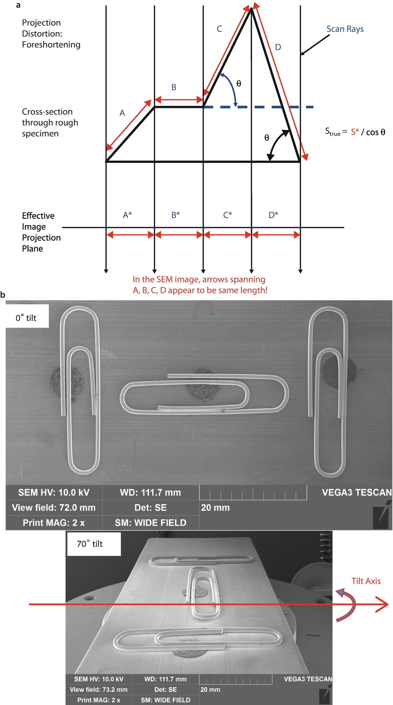
a Schematic illustration of projection distortion of tilted surfaces. b Illustration of foreshortening of familiar objects, paper clips (*upper*) Large area image at 0 tilt; (*lower*) large area image at 70° tilt around a horizontal tilt axis. Note that parallel to the tilt axis, the paper clips have the same size, but perpendicular to the tilt axis severe foreshortening has occurred. The magnification also decreases significantly down the tilted surface, so the third paper clip appears smaller than the first (Images courtesy J. Mershon, TESCAN)

${L}_{\mathrm{image}}={L_{\mathrm{true}}}^{\ast}\kern0.50em \cos\ \theta$

(6.3)

For the situation shown in ◘ Fig. 6.7a, all four linear objects would have the same apparent size in the SEM image, but only one, object B, would be shown with the correct length since it lies in a plane perpendicular to the optic axis, while the true lengths of the other linear objects would be significantly underestimated. For the most severe case, object D, which lies on the most highly tilted surface with θ = 75°, the object is a factor of 3.9 longer than it appears in the image. The effect of foreshortening is dramatically illustrated in ◘ Fig. 6.7b, where familiar objects, paper clips, are seen in a wide area SEM image at 0° tilt and 70° tilt. At high tilt, the length of the first paper clip parallel to the tilt axis remains the same, while the second paper clip that is perpendicular to the tilt axis is highly foreshortened (Note that the third paper clip, which also lies parallel to the tilt axis, appears shorter than the first paper clip because the effective magnification decreases down the tilted surface). As shown schematically in ◘ Fig. 6.8, foreshortening causes a square to appear as a rectangle. The effect of foreshortening is shown for an SEM image of a planar copper grid in ◘ Fig. 6.9, where the square openings of the grid are correctly imaged at θ = 0° in ◘ Fig. 6.9a. When the specimen plane is tilted to θ = 45°, the grid appears to have rectangular openings, as shown in ◘ Fig. 6.9b, with the shortened side of the true squares running parallel to the y-axis, while the correctly sized side runs parallel to the x-axis, which is the axis of tilt. Some SEMs are equipped with a “tilt correction” feature in which the y-scan perpendicular to the tilt axis is decreased to compensate for the extended length (relative to the x-scan along the tilt axis) of the scan excursion on the tilted specimen, as shown schematically in ◘ Fig. 6.9c. Tilt correction creates the same magnification (i.e., the same pixel dimension) along orthogonal x- and y-axes, which restores the proper shape of the squares, as seen in ◘ Fig. 6.9c. However, this scan transformation is only correct for objects that lie in the plane of the specimen. ◘ Figure 6.9c also contains a spherical particle, which appears to be circular at θ = 0° and at θ = 45° without tilt correction, since the normal scan projects the intersection of the plane of the scan sphere as a circle. However, when tilt correction is applied at θ = 45°, the sphere now appears to be a distorted ovoid. Thus, applying tilt correction to the image of an object with three-dimensional features of arbitrary orientation will result in image distortions that will increase in severity with the degree of local tilt.

../images/271173_4_En_6_Chapter/271173_4_En_6_Fig8_HTML.png — Fig. 6.8
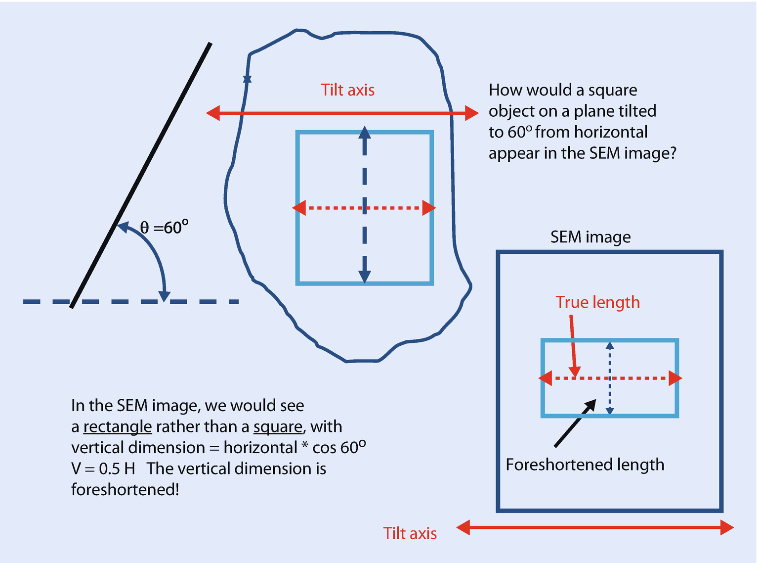
Effect of foreshortening of objects in a titled plane to distort square grid openings into *rectangles*

../images/271173_4_En_6_Chapter/271173_4_En_6_Fig9_HTML.png — Fig. 6.9
a SEM/E–T (positive) image of a copper grid with a polystyrene latex sphere; tilt = 0° (grid normal to electron beam). b Grid tilted to 45°; note the effect of foreshortening distorts the *square grid* openings into *rectangles*. c Grid tilted to 45°; “tilt correction” applied, but note that while the square grid openings are restored to the proper shape, the *sphere* is highly distorted

6.4.2 Image Defocusing (Blurring)

The act of focusing an SEM image involves adjusting the strength of the objective lens to bring the narrowest part of the focused beam cross section to be coincident with the surface. If the specimen has a flat, planar surface placed normal to the beam, then the situation illustrated in ◘ Fig. 6.10a will exist at sufficiently low magnification. ◘ Figure 6.10a shows the locations of the beam at the pixel centers in the middle of the squares and the effective sampling footprint. The sampling footprint consists of the contribution of the incident beam diameter (in this case finely focused to a diameter <10 nm) and the surface emergence area of the BSE and SE, which is controlled by the interaction volume. ◘ Figure 6.10a considers a situation of a low beam energy (e.g., 5 keV) and a high atomic number (e.g., Au). For these conditions, the beam sampling footprint only occupies a small fraction of each pixel area so that there is no possibility of overlap, i.e., sampling of adjacent pixels. Now consider what happens as the magnification is increased, i.e., the length l in Eq. (6.1) decreases while the pixel number, n, remains the same: the distance between pixel centers decreases, but the beam sampling footprint remains the same size for this particular material and beam landing energy. The situation shown in ◘ Fig. 6.10b for the original beam sampling footprint relative to the pixel spacing and four successive increases in magnification reveals that as the pixel spacing becomes smaller, the beam sampling footprint eventually leaks into the surrounding pixels, so that the beam no longer samples exclusively the region of a single pixel. Eventually, when enough pixels overlap, the observer will perceive this leakage as image defocusing or blurring. The reality and limitations of this situation become obvious when the microscopist seeks to perform high spatial resolution microscopy, a topic which will be covered in more depth in module 10 on high resolution SEM.

../images/271173_4_En_6_Chapter/271173_4_En_6_Fig10_HTML.png — Fig. 6.10
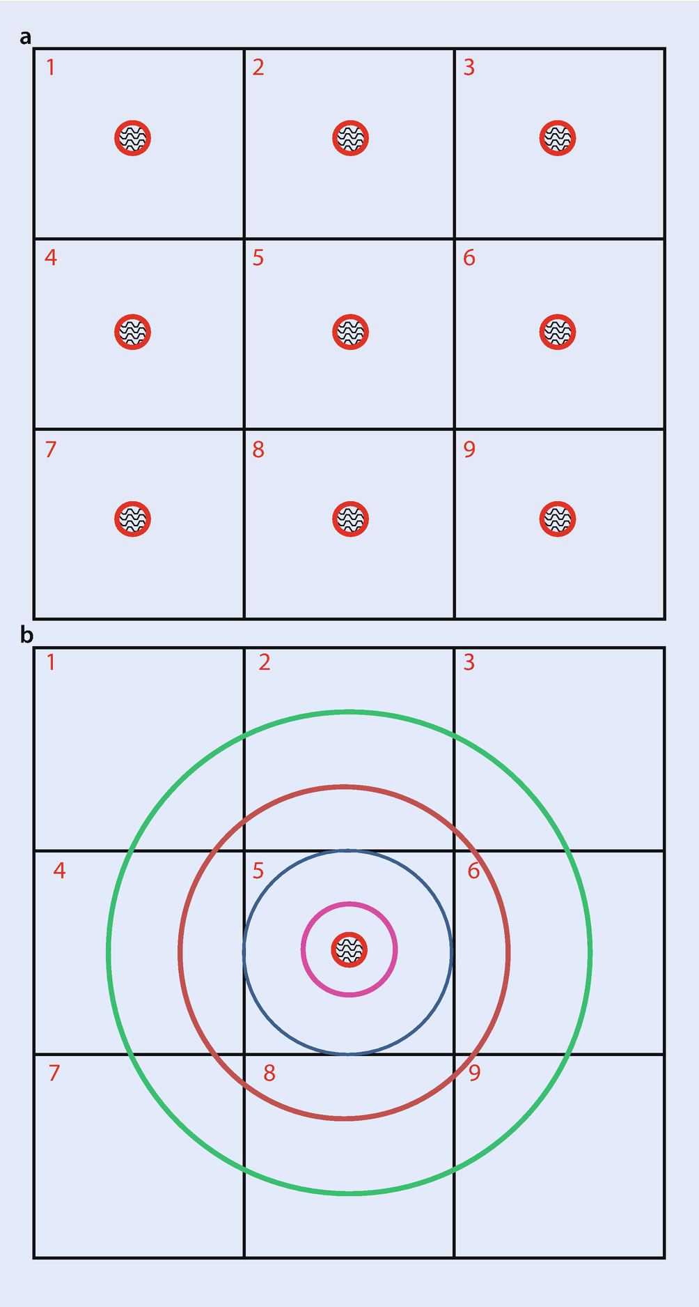
a The beam sampling footprint relative to the pixel spacing for a low magnification image with a low energy finely focused beam and a high atomic number target. b As the magnification is increased with fixed beam energy and target material, the beam sampling footprint (diameter and BSE-SE convolved) eventually fills the pixel and progressively leaks into adjacent pixels

The effects of blurring are also encountered in the trivial case when the objective lens is strengthened or weakened, which moves the minimum beam convergence along the vertical axis (either up or down), as shown schematically in ◘ Fig. 6.11a, increasing the size of the beam that encounters the specimen surface. The beam diameter that encounters the specimen surface will be larger in either case because of the finite convergence angle, α. As the beam samples progressively more adjacent pixels just due to the increase in beam size, and not dependent on the BSE-SE sampling footprint, the observer will eventually perceive the defocusing, and hopefully correct the situation!

../images/271173_4_En_6_Chapter/271173_4_En_6_Fig11_HTML.jpg — Fig. 6.11
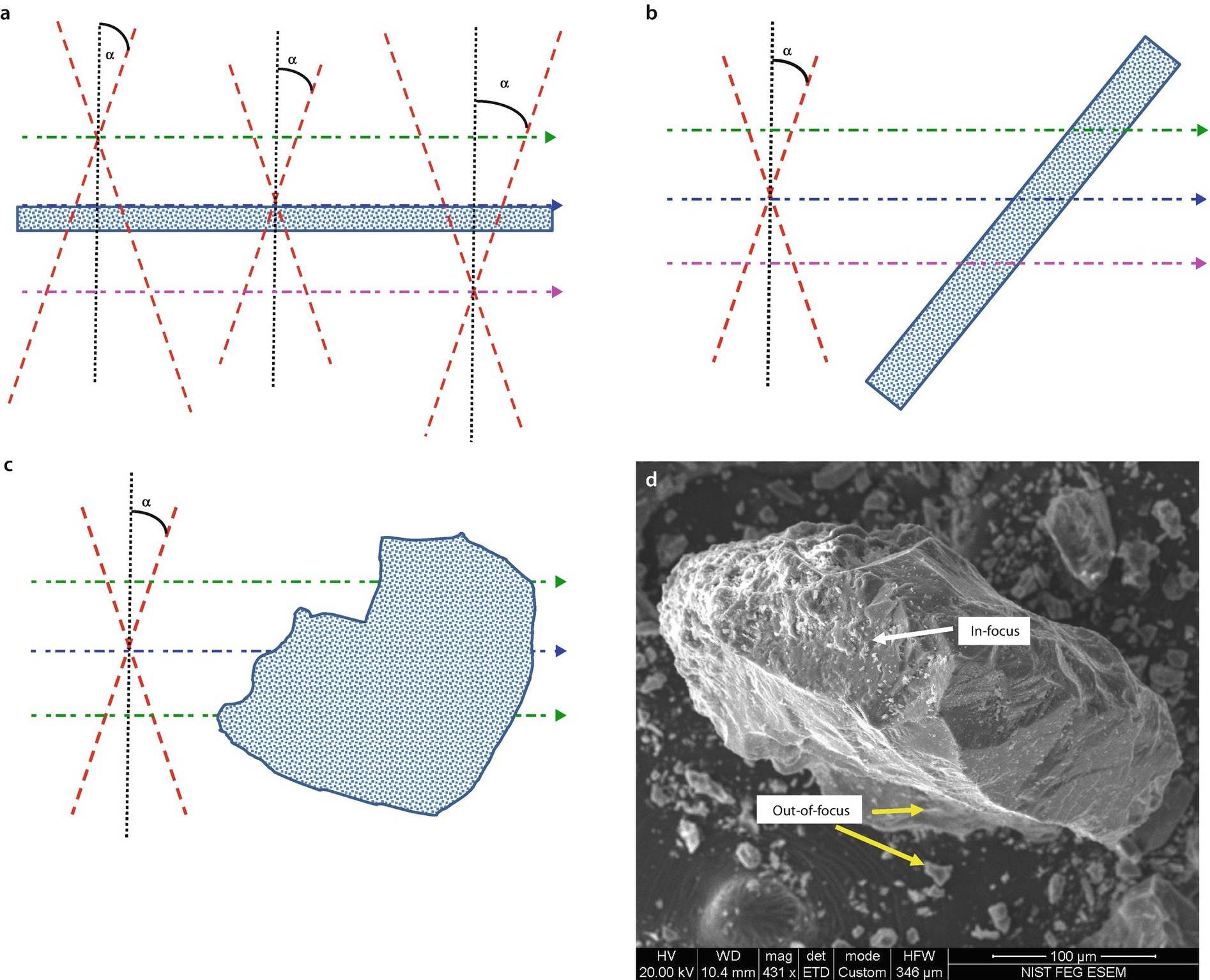
a Trivial example of optimal lens strength (focused at *blue plane*) and defocusing caused by selecting the objective lens strength too high (focused at *green plane*) and too low (focused at *magenta plane*) relative to the specimen surface. b Effect of a tilted planar surface. The beam is scanned with fixed objective lens strength, so that different beam diameters encounter the specimen at different distances along the optic axis. c Effects similar to ◘ Fig. 6.11b but for a three-dimensional specimen of arbitrary shape. d An imaging situation corresponding to ◘ Fig. 6.11c: coated fragments of Mt. St. Helens ash mounted on conducting tape and imaged under high vacuum at E ₀ = 20 keV with an E–T (positive) detector

Defocusing is also encountered when the specimen has features that extend along the optic axis. For example, defocusing may be encountered when planar specimens are tilted or rough topographic specimens are examined, even at low magnifications, i.e., large scanned areas, as illustrated schematically in ◘ Fig. 6.11b, c. In these situations, the diameter of the converged beam that encounters the specimen depends on the distance of the feature from the bottom of the objective lens and the convergence angle of the beam, α. Because the beam is focused to a minimum diameter at a specific distance from the objective lens, the working distance W, any feature of the specimen that the scanned beam encounters at any other distance along the optic axis will inevitably involve a larger beam diameter, which can easily exceed the sampling footprint of the BSE and SE. ◘ Figure 6.11d shows an image of Mt. St. Helens volcanic ash particles where the top of the large particle is in good focus, but the focus along the sides of the particles deteriorates into obvious blurring, as also occurs for the small particles dispersed around the large particle on the conductive tape support. This defocus situation can only be improved by reducing the convergence angle, α, as described in Depth-of-Field Mode operation.

6.5 Making Measurements on Surfaces With Arbitrary Topography: Stereomicroscopy

By operating in Depth-of-Field Mode, which optimizes the choice of the beam convergence angle, α, a useful range of focus along the optic axis can be established that is sufficient to render effective images of complex three-dimensional objects. ◘ Figure 6.12 shows an example of a specimen (metal fracture surface) with complex surface topography. The red arrows mark members of a class of flat objects. If the microscopist’s task is to measure the size of these objects, the simple linear measurement that is possible in a single SEM image is subject to large errors because the local tilt of each feature is different and unknown, which corresponds to the situation illustrated in ◘ Fig. 6.7. Although lost in a single two-dimensional image, the third dimension of an irregular surface can be recovered by the technique of stereomicroscopy.

../images/271173_4_En_6_Chapter/271173_4_En_6_Fig12_HTML.jpg — Fig. 6.12
SEM/E–T (positive) image of a metal fracture surface. The red arrows designate members of a class of flat objects embedded in this surface

6.5.1 Qualitative Stereomicroscopy

The human visual process creates the perception of depth and the three-dimensional character of objects by combining the separate two-dimensional views provided by the left eye and the right eye to create a fused image, as shown in ◘ Fig. 6.13. The angular difference between the eyes creates two distinct views containing parallax information, which is the horizontal shift (relative to a vertical axis) of a feature common to the two separate views. The parallax is the critical information that the brain uses to create the sensation of depth in the fused image: the larger the parallax, the closer the object is to the viewer. To create a similar sensation of depth, SEM stereomicroscopy operates by mimicking the human visual process and creating two angularly separated views of the specimen with parallax information. In SEM imaging, the electron beam is the “eye of the observer” (see the “Image Interpretation” module), so the two required images for stereo imaging must be obtained by either changing the orientation of the beam relative to the specimen (beam rocking method), or by changing the orientation of the specimen relative to the fixed electron beam (specimen tilting method). An appropriate image separation method such as the anaglyph technique (e.g., using red and cyan filters to view color-coded images) then presents the each member of the image pair to the left or right eye so that the viewer’s natural imaging process will create a fused image that reveals the third dimension. (Note that there is a fraction of the population for whom this process is not effective at creating the sense of viewing a three-dimensional object.)

../images/271173_4_En_6_Chapter/271173_4_En_6_Fig13_HTML.png — Fig. 6.13
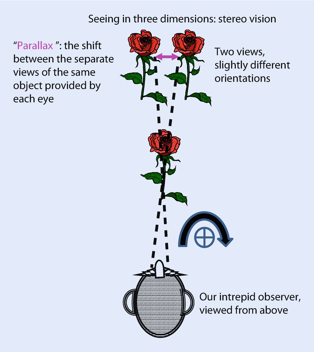
Schematic illustration of an observer’s creation of a stereo view of an object. Note that the parallax (shift between the two views) is across a vertical axis

6.5.1.1 Fixed beam, Specimen Position Altered

Parallax can be created by changing the specimen tilt relative to the optic axis (beam) by recording two images with a difference in tilt angle ranging from 2^° to 10^°. The specific value depends on the degree of topography of the specimen, and the optimum choice may require a trial-and-error approach. Weak topography will generally require a larger tilt difference to create a suitable three-dimensional effect. However, if the tilt angle difference between the images is made too large, it may not be possible for a viewer to successfully fuse the images and visualize the topography, especially for large-scale topography.

A suitable procedure to achieve SEM stereomicroscopy with a fixed beam by tilting the specimen has the following steps:

1.
Determine where the tilt axis lies in the SEM image. The eventual images must be presented to the viewer with horizontal parallax (i.e., all the shift between the two images must be across a vertical axis), so the tilt axis must be oriented vertically. The images can be recorded and rotated appropriately within image processing software such as ImageJ-Fiji, or the scan rotation function of the SEM can be used to orient the tilt axis along the vertical. In either case, note the location of the Everhart–Thornley detector in the image, which will provide the general sense of illumination. Ideally, the position of the E–T detector should be at the top of the image. However, after image rotation to orient the tilt axis vertically, the effective position of the Everhart-Thornley detector is likely to be different from this ideal 12-o’clock position (top center of image).
2.
Record an image of the area of interest at the low tilt angle, for example, stage tilt = 0^°.
3.
Using this image as a reference, increase the tilt angle to the desired value, e.g., stage tilt = 5^°, while maintaining the location of the field of view. Depending on the mechanical sophistication of the specimen stage, changing the tilt may cause the field of view to shift laterally, requiring continual relocation of the desired field of view during the tilting process to avoid losing the area of interest, especially at high magnification on specimens with complex topography.
4.
The vertical position of the specimen may also shift during tilting. To avoid introducing rotation in the second (high tilt image) by changing the objective lens strength to re-focus, the vertical stage motion (z-axis) should be used to refocus the image. After careful adjustment of the x-y-z position of the stage using the low tilt image to locate the area of interest, record this high tilt image.
5.
Within the image-processing software, assign the low tilt image to the RED image channel and the high tilt image to the CYAN (GREEN-BLUE channels combined, or the individual GREEN or BLUE image channels, depending on the type of anaglyph viewing filters available). Apply the image fusion function to create the stereo image, and view this image display with appropriate red (left eye) and blue (right eye) glasses. Note: The image-processing software may allow fine scale adjustments (shifts and/or rotations) to improve the registration of the images. This procedure is illustrated in ◘ Fig. 6.14 for the “Anaglyph Maker STEREOEYE” software (► http://www.stereoeye.jp/index_e.html). Examples of “stereo pairs” created in this manner are shown in ◘ Fig. 6.15 (a particle of ash from the Mt. St. Helens eruption) and ◘ Fig. 6.16 (gypsum crystals from cement).
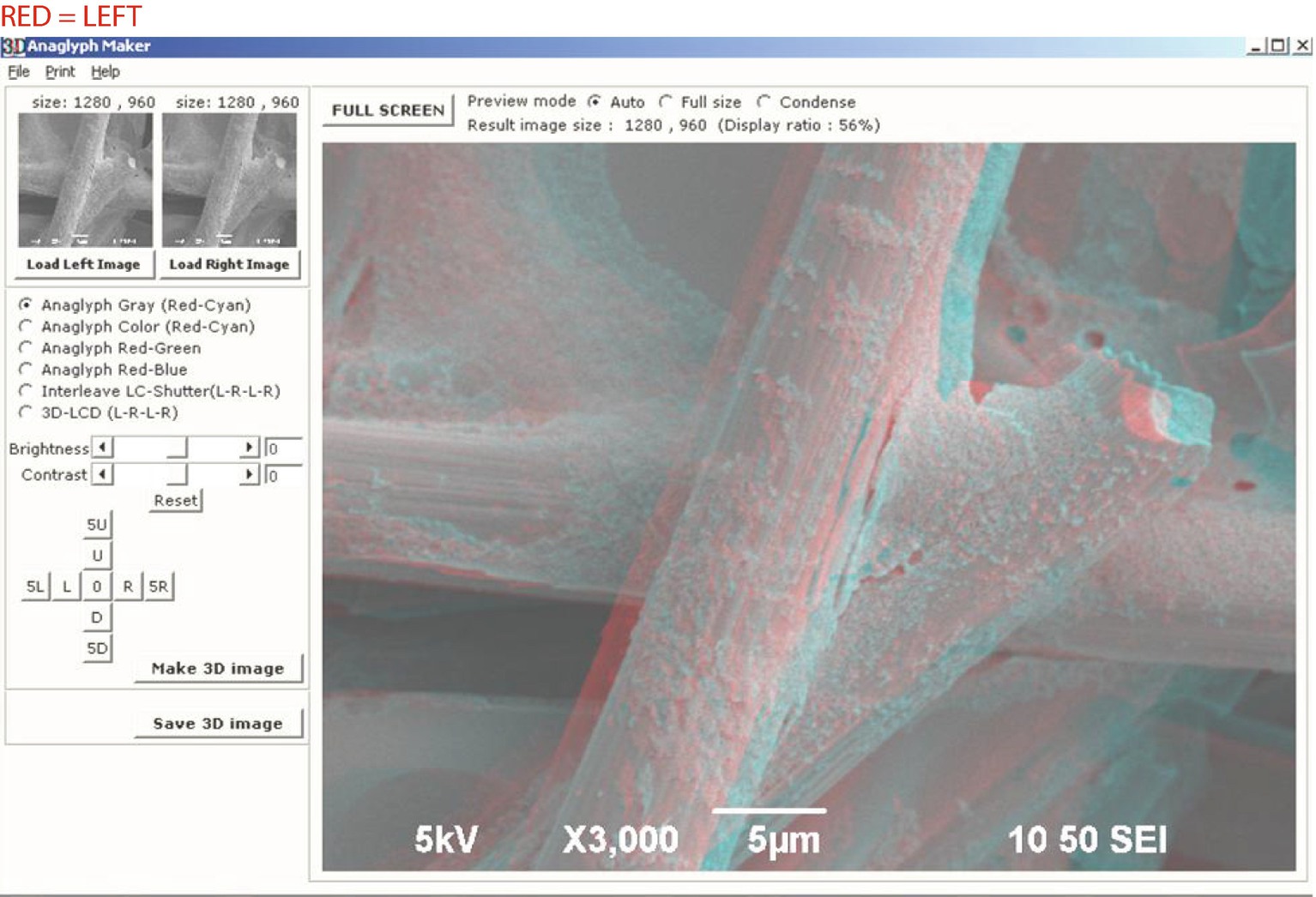Fig. 6.14
Illustration of the main page of the “Anaglyph Maker STEREOEYE” software (► http://www.stereoeye.jp/index_e.html) showing the windows where the left (low tilt) and right (high tilt) SEM/E–T (positive) images are selected and the resulting anaglyph (convention: red filter for the left eye). Note that brightness and contrast and fine position adjustments are available to the user. Specimen: ceramic fibers, coated with Au-Pd; E ₀ = 5 keV

Fig. 6.15
Anaglyph stereo presentation of SEM/E–T(positive) images (E ₀ = 20 keV) of a grain of Mt. St. Helens volcanic ash prepared by the stage tilting stereo method

Fig. 6.16
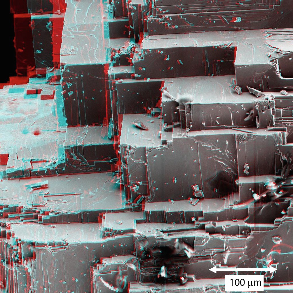
Anaglyph stereo presentation of SEM/E–T(positive) images (E ₀ = 20 keV) of a grain of gypsum crystals prepared by the stage tilting stereo method

Note

While usually successful, this SEM stereomicroscopy “recipe” may not produce the desired stereo effect on your particular instrument. Because of differing conventions for labeling tilt motions or due to unexpected image rotation applied in the software, the sense of the topography may be reversed (e.g., a topographic feature that is an “inner” falsely becomes an “outer” and vice versa). It is good practice when first implementing stereomicroscopy with an SEM to start with a simple specimen with known topography such as a coin with raised lettering or a scratch on a flat surface. Apply the procedure above and inspect the results to determine if the proper sense of the topography has been achieved in the resulting stereo pair. If not, be sure the parallax shift is horizontal, that is, across a vertical axis (if necessary, use software functions to rotate the images to vertically orient the tilt axis). If the tilt axis is vertical but the stereo pair still shows the wrong sense of the topography, try reversing the images so the “high tilt” image is now viewed by the left eye and the “low tilt” image viewed by the right eye. Once the proper procedure has been discovered to give the correct sense of the topography on a known test structure, follow this convention for future stereomicroscopy work. (Note: A small but significant fraction of observers find it difficult to fuse the images to form a stereo image.)

6.5.1.2 Fixed Specimen, Beam Incidence Angle Changed

The beam incidence angle relative to the specimen can be changed by a small value by means of a deflection in the final stage of the scan to create the two distinct views needed to achieve the stereo effect. An example of a stereo pair created in this manner is shown in ◘ Fig. 6.17 for a fractured fragment of galena. By applying the two beam tilts to alternate image scans at high rate, “live” 3D SEM imaging can be achieved that is nearly “flicker free.” By eliminating the need for mechanical stage motion as well as avoiding problems which frequently occur due to shifting of the area of interest during mechanical tilting, the speed of the beam tilting method makes it very powerful for studying complex topography. This is especially true at high magnification when the act of mechanical stage tilting is more likely to cause significant lateral shifting of the specimen, rendering the mechanical stage tilt stereo method tedious. An example of a stereo pair for a silver crystal produced with the beam tilt method at higher magnification is shown in ◘ Fig. 6.18.

../images/271173_4_En_6_Chapter/271173_4_En_6_Fig17_HTML.jpg — Fig. 6.17
Anaglyph stereo presentation of SEM/E–T(positive) images (E ₀ = 15 keV) of a fractured galena crystal prepared by the beam tilting stereo method

../images/271173_4_En_6_Chapter/271173_4_En_6_Fig18_HTML.png — Fig. 6.18
Anaglyph stereo presentation of SEM/E–T(positive) images (E ₀ = 15 keV) of a silver crystal prepared by the beam tilting stereo method

6.5.2 Quantitative Stereomicroscopy

Quantitation of the topography in SEM micrographs can be carried out by calculating the Z-coordinate of the feature from measurements of the x- and y-coordinates in the members of a stereo pair, as illustrated schematically in ◘ Fig. 6.19 (Boyde 1973, 1974a,b; Wells 1974). This procedure can be accomplished even if the operator is not personally able to perceive the qualitative stereo effect using the anaglyph or other methods to present the two images.

../images/271173_4_En_6_Chapter/271173_4_En_6_Fig19_HTML.png — Fig. 6.19
Schematic diagram of the procedure for making quantitative stereo measurements

1.
The first step is to record a stereo pair with tilt angles θ₁ and θ₂ and with the tilt axis placed in a vertical orientation in the images. The difference in tilt angle between the members of the stereo pair is a critical parameter:
$\varDelta \theta ={\theta}_2-{\theta}_1$

(6.4)
2.
A set of orthogonal axes is centered on a recognizable feature, as shown in the schematic example in ◘ Fig. 6.19. This point will then be arbitrarily assigned the X-, Y-, Z-coordinates (0, 0, 0) and all subsequent height measurements will be with respect to this point. The axes are selected so that the y-axis is parallel to the tilt axis and the x-axis is perpendicular to the tilt axis.
3.
For the feature of interest, the (X, Y)-coordinates are measured in the Left (X _L, Y _L) and Right (X _R, Y _R) members of the stereo pair using the calibrated distance marker. The parallax, P, of a feature is given by
$P=\left({X}_{\mathrm{L}}-{X}_{\mathrm{R}}\right)$

(6.5)

With this convention, points lying above the tilt axis will have positive parallax values P. Note that as an internal consistency check, Y _L = Y _R if the y-axis has been properly aligned with the tilt axis.
4.
For SEM magnifications above a nominal value of 100×, the scan angle will be sufficiently small that it can be assumed that the scan is effectively moving parallel to the optic axis, which enables the use of simple formulas for quantification. With reference to the fixed point (0, 0, 0), the three-dimensional coordinates X ₃, Y ₃, Z ₃ of the chosen feature are given by
${Z}_3=P/\left[2\ \sin\ \left(\varDelta \theta /2\right)\right]$

(6.6)

${X}_3=\left(P/2\right)+{X}_{\mathrm{L}}={X}_{\mathrm{R}}-\left(P/2\right)$

(6.7)

(Note that Eq. (6.7) provides a self-consistency check for the X₃ coordinate.)
${Y}_3={Y}_{\mathrm{L}}={Y}_{\mathrm{R}}$

(6.8)

Note that if the measured coordinates y _L and y _R are not the same then this implies that the tilt axis is not accurately parallel to Y and the axes must then be rotated to correct this error.
By measuring any two points with coordinates, (X _M, Y _M, Z _M) and (X _N, Y _M, Z _M), the length L of the straight line connecting the points is given by
$L=\mathrm{SQRT}\left[{\left({X}_{\mathrm{M}}-{X}_{\mathrm{N}}\right)}^2+{\left({Y}_{\mathrm{M}}-{Y}_{\mathrm{N}}\right)}^2+{\left({Z}_{\mathrm{M}}-{Z}_{\mathrm{N}}\right)}^2\right]$

(6.9)

6.5.2.1 Measuring a Simple Vertical Displacement

The stereo pair in ◘ Fig. 6.20a illustrates a typical three-dimensional measurement problem: for this screw thread, how far above or below is the feature circled in green relative to the feature circled in yellow? The left image (low tilt, θ = 0°) and right image (high tilt, θ = 5°) are prepared according to the convention described above and oriented so that the tilt axis is vertical. It is good practice to inspect the stereo pair with the anaglyph method shown in ◘ Fig. 6.14 to ensure that the stereo pair is properly arranged, and to qualitatively assess the nature of the topography, i.e., determine how features are arranged relative to each other, as shown for this image of the screw thread in ◘ Fig. 6.20a. In ◘ Fig. 6.20b, a set of x- (horizontal) and y- (vertical) axes are established in each image centered on the feature in the yellow circle, which is assigned the origin of coordinates (0, 0, 0). Using this coordinate system, measurements are made of the feature of interest (within the green circle) in the left (X _L = 144 μm, Y _L = −118 μm) and right (X _R = 198 μm, Y _R = −118 μm) images. The parallax P is then

../images/271173_4_En_6_Chapter/271173_4_En_6_Fig20_HTML.png — Fig. 6.20
a Stereo pair of a machined screw thread—SEM/E–T(positive) images; E ₀ = 20 keV. b Stereo pair with superimposed axes for measurement of coordinates needed for quantitative stereomicroscopy calculations

$P={X}_{\mathrm{L}}-{X}_{\mathrm{R}}=144\ \mu \mathrm{m}-198\ \mu \mathrm{m}=-54\ \mu \mathrm{m}$

(6.10)

Note that the sign of the parallax is negative, which means that the green circle feature is below the yellow circle feature, a result that is confirmed by the qualitative inspection of the stereo pair in ◘ Fig. 6.20a. Inserting these values into Eq. (6.6), the Z-coordinate of the end of the green circle feature relative to the yellow circle feature is calculated to be:

$\begin{array}{l}{Z}_3=P/\left[2\ \sin\ \left(\varDelta \theta /2\right)\right]\ \\ {}=-54\ \mu \mathrm{m}/\left[2\ \sin \left({5}^{{}^{\circ}}/2\right)\right]\ \\ {}=-619\ \mu \mathrm{m}\end{array}$

(6.11)

Thus, the feature in the green circle is 619 μm below the feature in the yellow circle at the origin of coordinates. The uncertainty budget for this measurement consists of the following components:

1.
Scale calibration error: with the careful use of a primary or secondary dimensional artifact, this uncertainty contribution can be reduced to 1 % relative or less.
2.
Measurement of the feature individual coordinates: The magnitude of this uncertainty contribution depends on how well the position of a feature can be recognized and on the separation of the features of interest. By selecting a magnification such that the features whose vertical separation is to be measured span at least half of the image field, the uncertainty in the individual coordinates should be approximately 1 % relative, and in the difference of X-coordinates (X _L–X _R) about 2 % relative. For closely spaced features, the magnitude of this uncertainty contribution will increase.
3.
Uncertainty in the individual tilt settings: The magnitude of this uncertainty is dependent on the degree of backlash in the mechanical stage motions. Backlash effects can be minimized by selecting the initial (low) tilt value to correspond to a well-defined detent position if the mechanical stage is so designed, such as a physical stop at 0° tilt. With a properly maintained mechanical stage, the uncertainty in the tilt angle difference Δθ is estimated to be approximately 2 % for Δθ = 5⁰, with the relative uncertainty increasing for smaller values of Δθ.
4.
Considering all of these sources of uncertainty, the measurement should be assigned an overall uncertainty of ±5 % relative.

Open Access This chapter is licensed under the terms of the Creative Commons Attribution-NonCommercial 2.5 International License (http://creativecommons.org/licenses/by-nc/2.5/), which permits any noncommercial use, sharing, adaptation, distribution and reproduction in any medium or format, as long as you give appropriate credit to the original author(s) and the source, provide a link to the Creative Commons license and indicate if changes were made.

The images or other third party material in this chapter are included in the chapter's Creative Commons license, unless indicated otherwise in a credit line to the material. If material is not included in the chapter's Creative Commons license and your intended use is not permitted by statutory regulation or exceeds the permitted use, you will need to obtain permission directly from the copyright holder.

References

Boyde A (1973) Quantitative photogrammetric analysis and qualitative stereoscopic analysis of SEM images. J Microsc 98:452Crossref
Boyde A (1974a) A stereo-plotting device for SEM micrographs and a real time 3-D system for the SEM. In: Johari O (ed) SEM/1974. IIT Research Institute, Chicago, p 93
Boyde A (1974b) Photogrammetry of stereo pair SEM images using separate measurements from the two images. In: Johari O (ed) SEM/1974. IIT Research Institute, Chicago, p 101
Postek MT, Vladar AE, Ming B, Bunday B (2014) Documentation for Reference Material (RM) 8820: a versatile, multipurpose dimensional metrology calibration standard for scanned particle beam, scanned probe, and optical microscopy. NIST Special Publication 1170 ► https://www-s.nist.gov/srmors/view_detail.cfm?srm=8820
Wells O (1974) Scanning electron microscopy. McGraw-Hill, New York

6. Image Formation