CHAPTER 11
Beating It into Submission

There is more to say about dealing with tests that don’t produce the results you want. I think about this as a critical point in development, one in which you take the path that gives you the best chance of success, or you overfit the data so that there is no chance that the end product will work.

FIXING LOSING PERIODS

When you get disappointing results, you will look specifically at the trades, or sequence of trades, that caused the loss. Would a different stop-loss help? Were prices too volatile? Did you enter following a trade with a very large profit? Was this a short sale in a rising market? All of these questions seem valid, so why is there a problem?

It all depends on how you view the results based on those changes. For example, it’s a problem if:

• The change corrects only one trade.
• The change affects only one market.
• The results of an optimization show higher peak returns using some parameters, but lower returns using other parameters. That is, profits are concentrated in one area at the cost of other areas.
• The new results are unreasonably good.

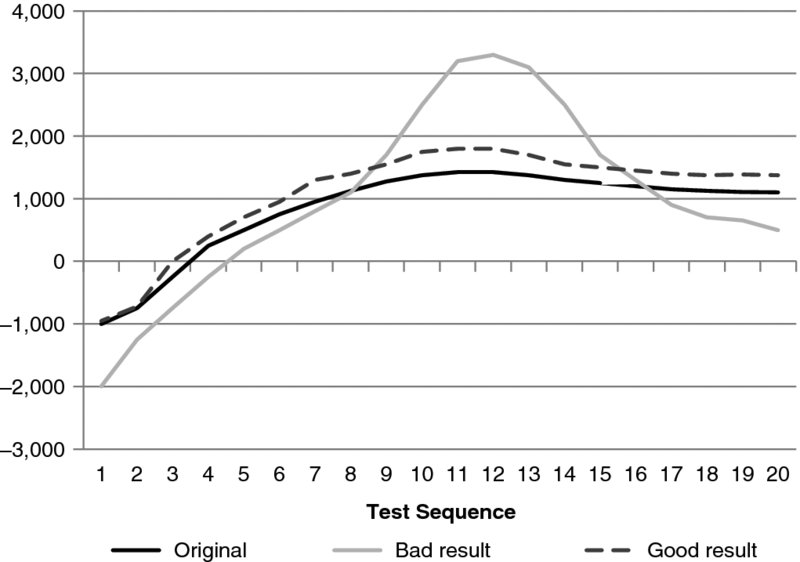
The third point, changing the pattern of results, needs to be clear. Consider the test results shown in Figure 11.1. The original test results are the dark line, going from negative 1,000, presumably the shortest calculation period, to 1,425 at the peak, and down to 1,100 at the right, the slowest period. Note that the results flatten out on the right because the percentage difference in the calculation periods get smaller and the results are similar.

FIGURE 11.1 Test Results Shown after Changes That Cause Concentration of Profits in the Center Compared to Changes That Improve All Test Results

After the rules are changed to improve some specific problems, the new test, shown by the gray line, results in much higher peak profits, while the wings of the results are worse than the original test. You may like this solution at first, but the concentration of improvement shows that a particular situation was targeted. This pattern can be found by quants using kurtosis, which essentially measures the peak. Normal kurtosis has the value of 3 (the shape of a standard bell curve), and anything above 6 is seen as a very narrow peak in the center and should be considered a problem.

By contrast, the “good” result shown in Figure 11.1 as a broken line improves most results in a more uniform manner. This is the ideal result, a change of rules that even improves the worst test results. A rule that achieves this result will be generalized, that is, it won’t focus on a particular trade, but on the nature of price movements. We’ll discuss this more in the sections that follow.

USE THE AVERAGE RESULTS

My own way of assessing success may not be attractive to many other traders, but I’ve never found a reason to do it differently. It requires that you first define the range of parameters that should work for your new strategy.

For example, if you are looking for the long-term trend, then calculation periods from 40 to 120, or 60 to 250, may be ranges that should work. If you are looking at a divergence pattern with a holding period of 3 to 8 days, then the pattern should be formed over 5 to 15 days. If you have an intraday breakout and a holding period of 3 days, then your profit targets should be in the range of 0.50 to 3.50 ATRs. You should not choose a wide range with the idea of looking at where the profits lie, then narrowing it down to include only the profitable area.

By defining the range in advance, you validate your idea of what works. If only 25% of the tests in your range turn out to be profitable, you need to rethink why you were wrong. The strategy is not doing what you expected.

Normally, you’ll be correct about the choice of the parameter test range and the results will look pretty good. The most important value will be the average of all tests, whether it’s net profits or the information ratio. The average result is also the most likely expected return in the future, much like economists forecast the mean (the average) one period ahead. The average is always the safest forecast.

The reasoning behind using the average is that we have a poor record of choosing a single parameter value from the test results that will perform each month going forward in exactly the way it did in the past. The results shown in a 10-year test may be the best net profit, but the way it got there might be erratic, with a sequence of losing months before a profitable run came along.

Consider the best result in a series of 100 tests. What is the likelihood that those parameters will give you the best result in the next month or year? I would argue that the best result is normally the least likely to perform well because it benefited from some unusual price movement, perhaps one or more price shocks. Given enough tests, one test is likely to be on the right side of the market when a surprise event drives prices sharply up or down. That event is not going to be repeated, so basing your parameter selection on an outlier will result in disappointing future performance.

Because I have never been successful at figuring out which specific parameters will perform best in the next month, I try to duplicate the average performance. That’s why I measure success by the average of all tests. To get an average result, you need to trade your strategy with a sample of different parameters, but no fewer than three, spread across the whole set of results. If we’re looking at a simple moving average method, I usually double the calculation period, for example, 30, 60, and 120 days. The percentage difference gives a better distribution. Then you trade each of the three subsystems with equal amounts. The more subsystems, the closer you get to the average.

Granted, the average result isn’t as glamorous as the best results from your tests, but they are more realistic. One of the goals of system development is to accurately predict both the returns and the risk of real trading. I think this approach comes close.

SQUEEZING THE LIFE OUT OF A SYSTEM

One of my favorite short-term systems is the 3-Day Trade. It’s not actually three days, but it has a 3-day setup period. The rules for a sell signal go as follows:

• Prices close up two days in a row.
• Sell the next open if higher than today’s close or sell the next close if it’s higher than today’s close.
• Exit on the close of the following day.

It takes three days to trigger the entry and the trade is held for two days if you enter on the open and one day if you enter on the close. The rules are symmetric, so that you buy after two lower closes and a lower open or lower close.

In the spirit of improvement, we also can add the rules:

• Take profits if prices move 2 ATRs from the entry.
• Enter short sales any time that prices spike 2.5 ATRs and the price closes in the upper 25% of the daily range.

Both additional rules are generalized based on volatility, so they qualify according to our guidelines, which are discussed more in the next section. The first extra rule, taking profits, will capture any fast, large, and favorable moves in our direction. When we operate in the short-term arena, we expect a lot of market noise, so capturing a profit based on some news announcement will be to our advantage.

The second rule, entering on a price spike without waiting for the 2-day setup, is also reacting to market noise. This rule works best for equity index markets, which tend to have more noise than other sectors. A volatility of 2.5 times the normal volatility is a noticeably strong or weak day, and prices closing near the top or bottom of that range provides the opportunity for a reversal the next day.

Both rules improve results in general over a wide selection of equity index markets and sufficient data. So far, so good.

But there is more. Floor traders have always believed that, during a trend, say an upward move, prices will open higher on Monday, then reverse Tuesday or Wednesday. Fridays may see selling pressure when some traders exit their positions to go home flat on the weekend. So the days of the week may be important.

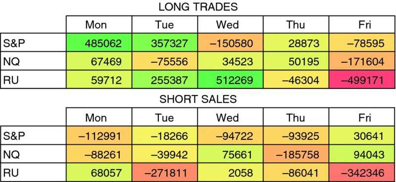
Finding out if this pattern is true doesn’t require a change of rules, just a way of adding the returns for long and short sales by the day of the week. Using the original rules, plus the two extra ones, we can test three of the primary equity index futures markets, the emini S&P, NASDAQ, and the small caps, the Russell 2000. Figure 11.2 shows the profits and losses by day of the week from 1990 through May 2015.

FIGURE 11.2 Results by Day of the Week from 1990 for the S&P, NASDAQ, and Russell 2000 Futures

The results show that Monday is consistently good for buying all three index futures. Mondays and Tuesdays are good for the S&P, and Monday, Tuesday, and Wednesday are excellent for the Russell. Friday is also good for selling the S&P and NQ. Those results seem to confirm the patterns expressed by the floor traders.

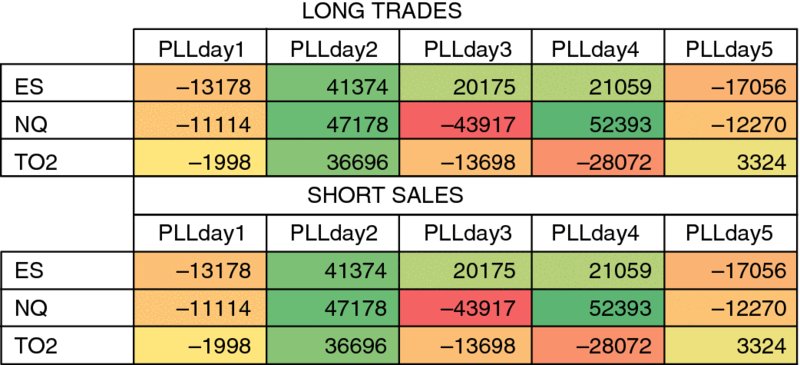
But this isn’t the whole picture. Let’s look at a more recent period, one year, starting in May 2014, shown in Figure 11.3. While Monday was consistently good for the entire period from 1990, it lost money during the past year. However, Tuesdays were consistently successful for both long and short positions. Thursdays are now very good for the S&P and NQ, even better than the longer test, but the best short sales have changed completely, shifting from Friday to Thursday.

FIGURE 11.3 Results by Day from May 2014 for the S&P, NASDAQ, and Russell 2000 Futures.

If we look further into the pattern of returns for the past 3 and 5 years, we find that there is even more of a shift. There is no consistency in returns based on the day of the week, but we would not have known that unless we looked deeper into the test results.

The good news is that the results show net profits if you add all the days of the week and avoid short sales. That should not be a surprise because the stock market is biased to the long side.

The lesson to be learned is that a system can be good, but you cannot try to isolate its profitable or losing patterns with too much accuracy. We win because, in the big picture, the numbers are on our side.

GENERALIZING THE RULES

There are a number of techniques that work across both time and markets. They may improve the performance of a wide range of systems. The most important of these are based on volatility.

Volatility is measured by the equities industry as the standard deviation of the daily returns times the square root of 252. There is an example of that in Chapter 9. But a better measure is the average true range, also discussed in Chapter 9.

High Volatility

High volatility is associated with high risk, but many traders think that their systems perform better during periods of high volatility. For certain, nothing does well when prices aren’t moving, and arbitrage programs will benefit from larger per share returns when volatility causes the two legs to go farther apart. But is that the real benefit?

In many cases, the payout for identifying high volatility is the ability to reduce the risk. We know that high volatility is the same as high risk, but we don’t know that it will also result in high returns. In fact, it is not likely, especially for trend following. For trades taken when the volatility is high, we see higher risk but not necessarily higher returns. That translates into a lower information ratio, which is the way we measure a successful strategy.

For short-term traders, I find that annualized volatility over 45% to 50% is too high. It is easy to skip those trades because there are always more to come. For long-term traders, I would look at reducing your exposure. Most often, that’s the same as taking profits, then resetting when volatility returns to near normal.

We’ll look at this again in Chapter 13.

Low Volatility

Low volatility is more complex. Markets can be lethargic at low volatility, meandering up and down, not going anywhere. In commodities in which a low price in wheat or metals can mean that it is trading near the level of production costs, there may be an exodus of traders looking for something more exciting. Lower liquidity and unchanged fundamentals will result in sideways price moves at the same time as low volatility. In general, a market that has low volatility is a poor place to put your money, no matter what your strategy is.

But there is another important aspect of low volatility. For some markets, such as interest rates, it could mean a steady move in one direction. While the relationship of return to risk is very good, the returns are very small. For futures traders, especially hedge funds using macrotrend systems, those periods are usually leveraged up so that the returns are larger, even though risk is also higher. Without leveraging up, results would never achieve expectations.