1.10 Test-Drive: Using IPython and Jupyter Notebooks

In this section, you’ll test-drive the IPython interpreter²⁵ in two modes:

25. Before reading this section, follow the instructions in the Before You Begin section to install the Anaconda Python distribution, which contains the IPython interpreter.

• In interactive mode, you’ll enter small bits of Python code called snippets and immediately see their results.

• In script mode, you’ll execute code loaded from a file that has the .py extension (short for Python). Such files are called scripts or programs, and they’re generally longer than the code snippets you’ll do in interactive mode.

Then, you’ll learn how to use the browser-based environment known as the Jupyter Notebook for writing and executing Python code.²⁶

26. Jupyter supports many programming languages by installing their "kernels." For more information see https://github.com/jupyter/jupyter/wiki/Jupyter-kernels.

1.10.1 Using IPython Interactive Mode as a Calculator

Let’s use IPython interactive mode to evaluate simple arithmetic expressions.

Entering IPython in Interactive Mode

First, open a command-line window on your system:

• On macOS, open a Terminal from the Applications folder’s Utilities subfolder.

• On Windows, open the Anaconda Command Prompt from the start menu.

• On Linux, open your system’s Terminal or shell (this varies by Linux distribution).

In the command-line window, type ipython, then press Enter (or Return). You’ll see text like the following, this varies by platform and by IPython version:

Python 3.7.0 | packaged by conda-forge | (default, Jan 20 2019, 17:24:52)
Type 'copyright', 'credits' or 'license' for more information
IPython 6.5.0 -- An enhanced Interactive Python. Type '?' for help.

In [1]:

The text "In [1]:" is a prompt, indicating that IPython is waiting for your input. You can type ? for help or begin entering snippets, as you’ll do momentarily.

Evaluating Expressions

In interactive mode, you can evaluate expressions:

In [1]: 45 + 72
Out[1]: 117

In [2]:

After you type 45 + 72 and press Enter, IPython reads the snippet, evaluates it and prints its result in Out[1].²⁷ Then IPython displays the In [2] prompt to show that it’s waiting for you to enter your second snippet. For each new snippet, IPython adds 1 to the number in the square brackets. Each In [1] prompt in the book indicates that we’ve started a new interactive session. We generally do that for each new section of a chapter.

27. In the next chapter, you’ll see that there are some cases in which Out[] is not displayed.

Let’s evaluate a more complex expression:

In [2]: 5 * (12.7 - 4) / 2
Out[2]: 21.75

Python uses the asterisk (*) for multiplication and the forward slash (/) for division. As in mathematics, parentheses force the evaluation order, so the parenthesized expression (12.7 - 4) evaluates first, giving 8.7. Next, 5 * 8.7 evaluates giving 43.5. Then, 43.5 / 2 evaluates, giving the result 21.75, which IPython displays in Out[2]. Whole numbers, like 5, 4 and 2, are called integers. Numbers with decimal points, like 12.7, 43.5 and 21.75, are called floating-point numbers.

Exiting Interactive Mode

To leave interactive mode, you can:

• Type the exit command at the current In [] prompt and press Enter to exit immediately.

• Type the key sequence <Ctrl> + d (or <control> + d). This displays the prompt "Do you really want to exit ([y]/n)?". The square brackets around y indicate that it’s the default response—pressing Enter submits the default response and exits.

• Type <Ctrl> + d (or <control> + d) twice (macOS and Linux only).

Self Check

1. (Fill-In) In IPython interactive mode, you’ll enter small bits of Python code called       and immediately see their results.
   Answer: snippets.

2. In IPython       mode, you’ll execute Python code loaded from a file that has the .py extension (short for Python).
   Answer: script.

3. (IPython Session) Evaluate the expression 5 * (3 + 4) both with and without the parentheses. Do you get the same result? Why or why not?
   Answer: You get different results because snippet [1] first calculates 3 + 4, which is 7, then multiplies that by 5. Snippet [2] first multiplies 5 * 3, which is 15, then adds that to 4.

   In [1]: 5 * (3 + 4)
   Out[1]: 35
   
   In [2]: 5 * 3 + 4
   Out[2]: 19
   

1.10.2 Executing a Python Program Using the IPython Interpreter

In this section, you’ll execute a script named RollDieDynamic.py that you’ll write in Chapter 6. The .py extension indicates that the file contains Python source code. The script RollDieDynamic.py simulates rolling a six-sided die. It presents a colorful animated visualization that dynamically graphs the frequencies of each die face.

Changing to This Chapter’s Examples Folder

You’ll find the script in the book’s ch01 source-code folder. In the Before You Begin section you extracted the examples folder to your user account’s Documents folder. Each chapter has a folder containing that chapter’s source code. The folder is named ch##, where ## is a two-digit chapter number from 01 to 17. First, open your system’s command-line window. Next, use the cd (“change directory”) command to change to the ch01 folder:

• On macOS/Linux, type cd ~/Documents/examples/ch01, then press Enter.

• On Windows, type cd C:\Users\YourAccount\Documents\examples\ch01, then press Enter.

Executing the Script

To execute the script, type the following command at the command line, then press Enter:

ipython RollDieDynamic.py 6000 1

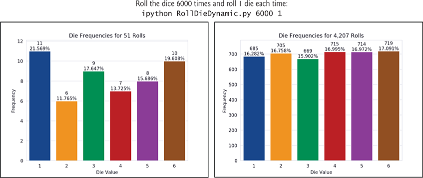
The script displays a window, showing the visualization. The numbers 6000 and 1 tell this script the number of times to roll dice and how many dice to roll each time. In this case, we’ll update the chart 6000 times for 1 die at a time.

For a six-sided die, the values 1 through 6 should each occur with “equal likelihood”—the probability of each is 1/6^th or about 16.667%. If we roll a die 6000 times, we’d expect about 1000 of each face. Like coin tossing, die rolling is random, so there could be some faces with fewer than 1000, some with 1000 and some with more than 1000. We took the screen captures on the next page during the script’s execution. This script uses randomly generated die values, so your results will differ. Experiment with the script by changing the value 1 to 100, 1000 and 10000. Notice that as the number of die rolls gets larger, the frequencies zero in on 16.667%. This is a phenomenon of the “Law of Large Numbers.”

Creating Scripts

Typically, you create your Python source code in an editor that enables you to type text. Using the editor, you type a program, make any necessary corrections and save it to your computer. Integrated development environments (IDEs) provide tools that support the entire software-development process, such as editors, debuggers for locating logic errors that cause programs to execute incorrectly and more. Some popular Python IDEs include Spyder (which comes with Anaconda), PyCharm and Visual Studio Code.

1.10-3 Full Alternative Text

Problems That May Occur at Execution Time

Programs often do not work on the first try. For example, an executing program might try to divide by zero (an illegal operation in Python). This would cause the program to display an error message. If this occurred in a script, you’d return to the editor, make the necessary corrections and re-execute the script to determine whether the corrections fixed the problem(s).

Errors such as division by zero occur as a program runs, so they’re called runtime errors or execution-time errors. Fatal runtime errors cause programs to terminate immediately without having successfully performed their jobs. Non-fatal runtime errors allow programs to run to completion, often producing incorrect results.

Self Check

1. (Discussion) When the example in this section finishes all 6000 rolls, does the chart show that the die faces appeared about 1000 times each?
   Answer: Most likely, yes. This example is based on random-number generation, so the results may vary. Because of this randomness, most of the counts will be a little more than 1000 or a little less.

2. (Discussion) Run the example in this section again. Do the faces appear the same number of times as they did in the previous execution?
   Answer: Probably not. This example uses random-number generation, so successive executions likely will produce different results. In Chapter 4, we’ll show how to force Python to produce the same sequence of random numbers. This is important for reproducibility—a crucial data-science topic you’ll investigate in the chapter exercises and throughout the book. You’ll want other data scientists to be able to reproduce your results. Also, you’ll want to be able to reproduce your own experimental results. This is helpful when you find and fix an error in your program and want to make sure that you’ve corrected it properly.

1.10.3 Writing and Executing Code in a Jupyter Notebook

The Anaconda Python Distribution that you installed in the Before You Begin section comes with the Jupyter Notebook—an interactive, browser-based environment in which you can write and execute code and intermix the code with text, images and video. Jupyter Notebooks are broadly used in the data-science community in particular and the broader scientific community in general. They’re the preferred means of doing Python-based data analytics studies and reproducibly communicating their results. The Jupyter Notebook environment actually supports many programming languages.

For your convenience, all of the book’s source code also is provided in Jupyter Notebooks that you can simply load and execute. In this section, you’ll use the JupyterLab interface, which enables you to manage your notebook files and other files that your notebooks use (like images and videos). As you’ll see, JupyterLab also makes it convenient to write code, execute it, see the results, modify the code and execute it again.

You’ll see that coding in a Jupyter Notebook is similar to working with IPython—in fact, Jupyter Notebooks use IPython by default. In this section, you’ll create a notebook, add the code from Section 1.10.1 to it and execute that code.

Opening JupyterLab in Your Browser

To open JupyterLab, change to the ch01 examples folder in your Terminal, shell or Anaconda Command Prompt (as in Section 1.10.2), type the following command, then press Enter (or Return):

jupyter lab

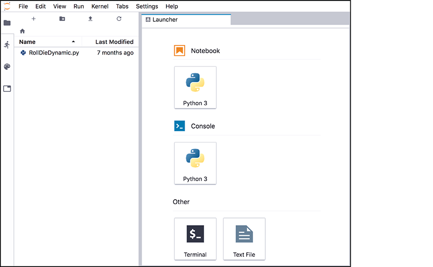
This executes the Jupyter Notebook server on your computer and opens JupyterLab in your default web browser, showing the ch01 folder’s contents in the File Browser tab

at the left side of the JupyterLab interface:

1.10-5 Full Alternative Text

The Jupyter Notebooks server enables you to load and run Jupyter Notebooks in your web browser. From the JupyterLab Files tab, you can double-click files to open them in the right side of the window where the Launcher tab is currently displayed. Each file you open appears as a separate tab in this part of the window. If you accidentally close your browser, you can reopen JupyterLab by entering the following address in your web browser

http://localhost:8888/lab

Creating a New Jupyter Notebook

In the Launcher tab under Notebook, click the Python 3 button to create a new Jupyter Notebook named Untitled.ipynb in which you can enter and execute Python 3 code. The file extension .ipynb is short for IPython Notebook—the original name of the Jupyter Notebook.

Renaming the Notebook

Rename Untitled.ipynb as TestDrive.ipynb:

1. Right-click the Untitled.ipynb tab and select Rename Notebook….

2. Change the name to TestDrive.ipynb and click RENAME.

The top of JupyterLab should now appear as follows:

Evaluating an Expression

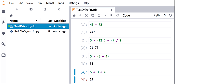
The unit of work in a notebook is a cell in which you can enter code snippets. By default, a new notebook contains one cell—the rectangle in the TestDrive.ipynb notebook—but you can add more. To the cell’s left, the notation [ ]: is where the Jupyter Notebook will display the cell’s snippet number after you execute the cell. Click in the cell, then type the expression

45 + 72

To execute the current cell’s code, type Ctrl + Enter (or control + Enter). JupyterLab executes the code in IPython, then displays the results below the cell:

Adding and Executing Another Cell

Let’s evaluate a more complex expression. First, click the + button in the toolbar above the notebook’s first cell—this adds a new cell below the current one:

Click in the new cell, then type the expression

5 * (12.7 - 4) / 2

and execute the cell by typing Ctrl + Enter (or control + Enter):

Saving the Notebook

If your notebook has unsaved changes, the X in the notebook’s tab will change to . To save the notebook, select the File menu in JupyterLab (not at the top of your browser’s window), then select Save Notebook.

Notebooks Provided with Each Chapter’s Examples

For your convenience, each chapter’s examples also are provided as ready-to-execute notebooks without their outputs. This enables you to work through them snippet-by-snippet and see the outputs appear as you execute each snippet.

So that we can show you how to load an existing notebook and execute its cells, let’s reset the TestDrive.ipynb notebook to remove its output and snippet numbers. This will return it to a state like the notebooks we provide for the subsequent chapters’ examples. From the Kernel menu select Restart Kernel and Clear All Outputs…, then click the RESTART button. The preceding command also is helpful whenever you wish to re-execute a notebook’s snippets. The notebook should now appear as follows:

From the File menu, select Save Notebook, then click the TestDrive.ipynb tab’s X button to close the notebook.

Opening and Executing an Existing Notebook

When you launch JupyterLab from a given chapter’s examples folder, you’ll be able to open notebooks from that folder or any of its subfolders. Once you locate a specific notebook, double-click it to open it. Open the TestDrive.ipynb notebook again now. Once a notebook is open, you can execute each cell individually, as you did earlier in this section, or you can execute the entire notebook at once. To do so, from the Run menu select Run All Cells. The notebook will execute the cells in order, displaying each cell’s output below that cell.

Closing JupyterLab

When you’re done with JupyterLab, you can close its browser tab, then in the Terminal, shell or Anaconda Command Prompt from which you launched JupyterLab, type Ctrl + c (or control + c) twice.

JupyterLab Tips

While working in JupyterLab, you might find these tips helpful:

• If you need to enter and execute many snippets, you can execute the current cell and add a new one below it by typing Shift + Enter, rather than Ctrl + Enter (or control + Enter).

• As you get into the later chapters, some of the snippets you’ll enter in Jupyter Notebooks will contain many lines of code. To display line numbers within each cell, select Show line numbers from JupyterLab’s View menu.

More Information on Working with JupyterLab

JupyterLab has many more features that you’ll find helpful. We recommend that you read the Jupyter team’s introduction to JupyterLab at:

https://jupyterlab.readthedocs.io/en/stable/index.html

For a quick overview, click Overview under GETTING STARTED. Also, under USER GUIDE read the introductions to The JupyterLab Interface, Working with Files, Text Editor and Notebooks for many additional features.

Self Check

1. (True/False) Jupyter Notebooks are the preferred means of doing Python-based data analytics studies and reproducibly communicating their results.
   Answer: True.

2. (Jupyter Notebook Session) Ensure that JupyterLab is running, then open your TestDrive.ipynb notebook. Add and execute two more snippets that evaluate the expression 5 * (3 + 4) both with and without the parentheses. You should see the same results as in Section 1.10.1’s Self Check Exercise 3.
   Answer: