15.3 Case Study: Classification with k-Nearest Neighbors and the Digits Dataset, Part 2

In this section, we continue the digit classification case study. We’ll:

• evaluate the k-NN classification estimator’s accuracy,

• execute multiple estimators and can compare their results so you can choose the best one(s), and

• show how to tune k-NN’s hyperparameter k to get the best performance out of a KNeighborsClassifier.

15.3.1 Metrics for Model Accuracy

Once you’ve trained and tested a model, you’ll want to measure its accuracy. Here, we’ll look at two ways of doing this—a classification estimator’s score method and a confusion matrix.

Estimator Method score

Each estimator has a score method that returns an indication of how well the estimator performs for the test data you pass as arguments. For classification estimators, this method returns the prediction accuracy for the test data:

In [35]: print(f'{knn.score(X_test, y_test):.2%}')
97.78%

The kNeighborsClassifier’s with its default k (that is, n_neighbors=5) achieved 97.78% prediction accuracy. Shortly, we’ll perform hyperparameter tuning to try to determine the optimal value for k, hoping that we get even better accuracy.

Confusion Matrix

Another way to check a classification estimator’s accuracy is via a confusion matrix, which shows the correct and incorrect predicted values (also known as the hits and misses) for a given class. Simply call the function confusion_matrix from the sklearn.metrics module, passing the expected classes and the predicted classes as arguments, as in:

In [36]: from sklearn.metrics import confusion_matrix

In [37]: confusion = confusion_matrix(y_true=expected, y_pred=predicted)

The y_true keyword argument specifies the test samples’ actual classes. People looked at the dataset’s images and labeled them with specific classes (the digit values). The y_pred keyword argument specifies the predicted digits for those test images.

Below is the confusion matrix produced by the preceding call. The correct predictions are shown on the diagonal from top-left to bottom-right. This is called the principal diagonal. The nonzero values that are not on the principal diagonal indicate incorrect predictions:

In [38]: confusion
Out[38]:
array([[45,  0,  0,  0,  0,  0,  0,  0,  0,  0],
       [ 0, 45,  0,  0,  0,  0,  0,  0,  0,  0],
       [ 0,  0, 54,  0,  0,  0,  0,  0,  0,  0],
       [ 0,  0,  0, 42,  0,  1,  0,  1,  0,  0],
       [ 0,  0,  0,  0, 49,  0,  0,  1,  0,  0],
       [ 0,  0,  0,  0,  0, 38,  0,  0,  0,  0],
       [ 0,  0,  0,  0,  0,  0, 42,  0,  0,  0],
       [ 0,  0,  0,  0,  0,  0,  0, 45,  0,  0],
       [ 0,  1,  1,  2,  0,  0,  0,  0, 39,  1],
       [ 0,  0,  0,  0,  1,  0,  0,  0,  1, 41]])

Each row represents one distinct class—that is, one of the digits 0–9. The columns within a row specify how many of the test samples were classified into each distinct class. For example, row 0:

[45, 0, 0, 0, 0, 0, 0, 0, 0, 0]

represents the digit 0 class. The columns represent the ten possible target classes 0 through 9. Because we’re working with digits, the classes (0–9) and the row and column index numbers (0–9) happen to match. According to row 0, 45 test samples were classified as the digit 0, and none of the test samples were misclassified as any of the digits 1 through 9. So 100% of the 0s were correctly predicted.

On the other hand, consider row 8 which represents the results for the digit 8:

[ 0, 1, 1, 2, 0, 0, 0, 0, 39, 1]

• The 1 at column index 1 indicates that one 8 was incorrectly classified as a 1.

• The 1 at column index 2 indicates that one 8 was incorrectly classified as a 2.

• The 2 at column index 3 indicates that two 8s were incorrectly classified as 3s.

• The 39 at column index 8 indicates that 39 8s were correctly classified as 8s.

• The 1 at column index 9 indicates that one 8 was incorrectly classified as a 9.

So the algorithm correctly predicted 88.63% (39 of 44) of the 8s. Earlier we saw that the overall prediction accuracy of this estimator was 97.78%. The lower prediction accuracy for 8s indicates that they’re apparently harder to recognize than the other digits.

Classification Report

The sklearn.metrics module also provides function classification_report, which produces a table of classification metrics⁵ based on the expected and predicted values:

5. http://scikit-learn.org/stable/modules/model_evaluation.html#precision-recall-and-f-measures.

In [39]: from sklearn.metrics import classification_report

In [40]: names = [str(digit) for digit in digits.target_names]

In [41]: print(classification_report(expected, predicted,
   ...:        target_names=names))
   ...:
            precision    recall    f1-score    support
      0          1.00      1.00        1.00         45
      1          0.98      1.00        0.99         45
      2          0.98      1.00        0.99         54
      3          0.95      0.95        0.95         44
      4          0.98      0.98        0.98         50
      5          0.97      1.00        0.99         38
      6          1.00      1.00        1.00         42
      7          0.96      1.00        0.98         45
      8          0.97      0.89        0.93         44
      9          0.98      0.95        0.96         43

micro avg        0.98      0.98        0.98        450
macro avg        0.98      0.98        0.98        450
weighted avg     0.98      0.98        0.98        450

In the report:

• precision is the total number of correct predictions for a given digit divided by the total number of predictions for that digit. You can confirm the precision by looking at each column in the confusion matrix. For example, if you look at column index 7, you’ll see 1s in rows 3 and 4, indicating that one 3 and one 4 were incorrectly classified as 7s and a 45 in row 7 indicating the 45 images were correctly classified as 7s. So the precision for the digit 7 is 45/47 or 0.96.

• recall is the total number of correct predictions for a given digit divided by the total number of samples that should have been predicted as that digit. You can confirm the recall by looking at each row in the confusion matrix. For example, if you look at row index 8, you’ll see three 1s and a 2 indicating that some 8s were incorrectly classified as other digits and a 39 indicating that 39 images were correctly classified. So the recall for the digit 8 is 39/44 or 0.89.

• f1-score—This is the average of the precision and the recall.

• support—The number of samples with a given expected value. For example, 50 samples were labeled as 4s, and 38 samples were labeled as 5s.

For details on the averages displayed at the bottom of the report, see:

http://scikit-learn.org/stable/modules/generated/sklearn.metrics.classification_report.html

Visualizing the Confusion Matrix

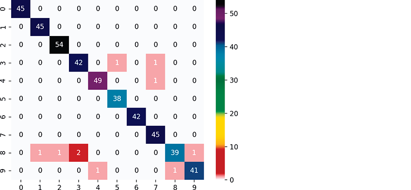
A heat map displays values as colors, often with values of higher magnitude displayed as more intense colors. Seaborn’s graphing functions work with two-dimensional data. When using a pandas DataFrame as the data source, Seaborn automatically labels its visualizations using the column names and row indices. Let’s convert the confusion matrix into a DataFrame, then graph it:

In [42]: import pandas as pd

In [43]: confusion_df = pd.DataFrame(confusion, index=range(10),
    ...: columns=range(10))
    ...:

In [44]: import seaborn as sns

In [45]: axes = sns.heatmap(confusion_df, annot=True,
    ...: cmap='nipy_spectral_r')
    ...:

The Seaborn function heatmap creates a heat map from the specified DataFrame. The keyword argument annot=True (short for “annotation”) displays a color bar to the right of the diagram, showing how the values correspond to the heat map’s colors. The cmap='nipy_spectral_r' keyword argument specifies which color map to use. We used the nipy_spectral_r color map with the colors shown in the heat map’s color bar. When you display a confusion matrix as a heat map, the principal diagonal and the incorrect predictions stand out nicely.

15.3-9 Full Alternative Text

Self Check

1. (Fill-In) A Seaborn ___________ displays values as colors, often with values of higher magnitude displayed as more intense colors.

   
   

   Answer: heat map.

2. (True/False) In a classification report, the precision specifies the total number of correct predictions for a class divided by the total number of samples for that class.

   
   

   Answer: True.

3. (Discussion) Explain row 3 of the confusion matrix presented in this section:

[ 0, 0, 0, 42, 0, 1, 0, 1, 0, 0]

Answer: The number 42 in column index 3 indicates that 42 3s were correctly predicted as 3s. The number 1 at column indices 5 and 7 indicates that one 3 was incorrectly classified as a 5 and one was incorrectly classified as a 7.

15.3.2 K-Fold Cross-Validation

K-fold cross-validation enables you to use all of your data for both training and testing, to get a better sense of how well your model will make predictions for new data by repeatedly training and testing the model with different portions of the dataset.K-fold cross-validation splits the dataset into k equal-size folds (this k is unrelated to k in the k-nearest neighbors algorithm). You then repeatedly train your model with k – 1 folds and test the model with the remaining fold. For example, consider using k = 10 with folds numbered 1 through 10. With 10 folds, we’d do 10 successive training and testing cycles:

• First, we’d train with folds 1–9, then test with fold 10.

• Next, we’d train with folds 1–8 and 10, then test with fold 9.

• Next, we’d train with folds 1–7 and 9–10, then test with fold 8.

This training and testing cycle continues until each fold has been used to test the model.

KFold Class

Scikit-learn provides the KFold class and the cross_val_score function (both in the module sklearn.model_selection) to help you perform the training and testing cycles described above. Let’s perform k-fold cross-validation with the Digits dataset and the KNeighborsClassifier created earlier. First, create a KFold object:

In [46]: from sklearn.model_selection import KFold

In [47]: kfold = KFold(n_splits=10, random_state=11, shuffle=True)

The keyword arguments are:

• n_splits=10, which specifies the number of folds.

• random_state=11, which seeds the random number generator for reproducibility.

• shuffle=True, which causes the KFold object to randomize the data by shuffling it before splitting it into folds. This is particularly important if the samples might be ordered or grouped. For example, the Iris dataset we’ll use later in this chapter has 150 samples of three Iris species—the first 50 are Iris setosa, the next 50 are Iris versicolor and the last 50 are Iris virginica. If we do not shuffle the samples, then the training data might contain none of a particular Iris species and the test data might be all of one species.

Using the KFold Object with Function cross_val_score

Next, use function cross_val_score to train and test your model:

In [48]: from sklearn.model_selection import cross_val_score

In [49]: scores = cross_val_score(estimator=knn, X=digits.data,
    ...: y=digits.target, cv=kfold)
    ...:

The keyword arguments are:

• estimator=knn, which specifies the estimator you’d like to validate.

• X=digits.data, which specifies the samples to use for training and testing.

• y=digits.target, which specifies the target predictions for the samples.

• cv=kfold, which specifies the cross-validation generator that defines how to split the samples and targets for training and testing.

Function cross_val_score returns an array of accuracy scores—one for each fold. As you can see below, the model was quite accurate. Its lowest accuracy score was 0.97777778 (97.78%) and in one case it was 100% accurate in predicting an entire fold:

In [50]: scores
Out[50]:
array([0.97777778, 0.99444444, 0.98888889, 0.97777778, 0.98888889,
       0.99444444, 0.97777778, 0.98882682, 1.        , 0.98324022])

Once you have the accuracy scores, you can get an overall sense of the model’s accuracy by calculating the mean accuracy score and the standard deviation among the 10 accuracy scores (or whatever number of folds you choose):

In [51]: print(f'Mean accuracy: {scores.mean():.2%}')
Mean accuracy: 98.72%

In [52]: print(f'Accuracy standard deviation: {scores.std():.2%}')
Accuracy standard deviation: 0.75%

On average, the model was 98.72% accurate—even better than the 97.78% we achieved when we trained the model with 75% of the data and tested the model with 25% earlier.

Self Check

1. (True/False) Randomizing the data by shuffling it before splitting it into folds is particularly important if the samples might be ordered or grouped.

   
   

   Answer: True.

2. (True/False) When you call cross_val_score to peform k-fold cross-validation, the function returns the best score produced while testing the model with each fold.

Answer: False. The function returns an array containing the scores for each fold. The mean of those scores is the estimator’s overall score.

15.3.3 Running Multiple Models to Find the Best One

It’s difficult to know in advance which machine learning model(s) will perform best for a given dataset, especially when they hide the details of how they operate from their users. Even though the KNeighborsClassifier predicts digit images with a high degree of accuracy, it’s possible that other scikit-learn estimators are even more accurate. Scikit-learn provides many models with which you can quickly train and test your data. This encourages you to run multiple models to determine which is the best for a particular machine learning study.

Let’s use the techniques from the preceding section to compare several classification estimators—KNeighborsClassifier, SVC and GaussianNB (there are more). Though we have not studied the SVC and GaussianNB estimators, scikit-learn nevertheless makes it easy for you to test-drive them by using their default settings.⁶ First, let’s import the other two estimators:

6. To avoid a warning in the current scikit-learn version at the time of this writing (version 0.20), we supplied one keyword argument when creating the SVC estimator. This argument’s value will become the default in scikit-learn version 0.22.

In [53]: from sklearn.svm import SVC

In [54]: from sklearn.naive_bayes import GaussianNB

Next, let’s create the estimators. The following dictionary contains key–value pairs for the existing KNeighborsClassifier we created earlier, plus new SVC and GaussianNB estimators:

In [55]: estimators = {
    ...:    'KNeighborsClassifier': knn,
    ...:    'SVC': SVC(gamma='scale'),
    ...:    'GaussianNB': GaussianNB()}
    ...:

Now, we can execute the models:

In [56]: for estimator_name, estimator_object in estimators.items():
...:      kfold = KFold(n_splits=10, random_state=11, shuffle=True)
...:      scores = cross_val_score(estimator=estimator_object,
...:          X=digits.data, y=digits.target, cv=kfold)
...:      print(f'{estimator_name:>20}: ' +
...:          f'mean accuracy={scores.mean():.2%}; ' +
...:          f'standard deviation={scores.std():.2%}')
...:
KNeighborsClassifier: mean accuracy=98.72%; standard deviation=0.75%
                 SVC: mean accuracy=99.00%; standard deviation=0.85%
          GaussianNB: mean accuracy=84.48%; standard deviation=3.47%

This loop iterates through items in the estimators dictionary and for each key-value pair performs the following tasks:

• Unpacks the key into estimator_name and value into estimator_object.

• Creates a KFold object that shuffles the data and produces 10 folds. The keyword argument random_state is particularly important here because it ensures that each estimator works with identical folds, so we’re comparing “apples to apples.”

• Evaluates the current estimator_object using cross_val_score.

• Prints the estimator’s name, followed by the mean and standard deviation of the accuracy scores’ computed for each of the 10 folds.

Based on the results, it appears that we can get slightly better accuracy from the SVC estimator—at least when using the estimator’s default settings. It’s possible that by tuning some of the estimators’ settings, we could get even better results. The KNeighborsClassifier and SVC estimators’ accuracies are nearly identical so we might want to perform hyperparameter tuning on each to determine the best.

Scikit-Learn Estimator Diagram

The scikit-learn documentation provides a helpful diagram for choosing the right estimator, based on the kind and size of your data and the machine learning task you wish to perform:

https://scikit-learn.org/stable/tutorial/machine_learning_map/index.html

Self Check

1. (True/False) You should choose the best estimator before performing your machine learning study.

   
   

   Answer: False. It’s difficult to know in advance which machine learning model(s) will perform best for a given dataset, especially when they hide the details of how they operate from their users. For this reason, you should run multiple models to determine which is the best for your study.

2. (Discussion) How would you modify the code in this section so that it would also test a LinearSVC estimator?

Answer: You’d import the LinearSVC class, add a key–value pair to the estimators dictionary ('LinearSVC': LinearSVC()), then execute the for loop, which tests every estimator in the dictionary.

15.3.4 Hyperparameter Tuning

Earlier in this section, we mentioned that k in the k-nearest neighbors algorithm is a hyperparameter of the algorithm. Hyperparameters are set before using the algorithm to train your model. In real-world machine learning studies, you’ll want to use hyperparameter tuning to choose hyperparameter values that produce the best possible predictions.

To determine the best value for k in the kNN algorithm, try different values of k then compare the estimator’s performance with each. We can do this using techniques similar to comparing estimators. The following loop creates KNeighborsClassifiers with odd k values from 1 through 19 (again, we use odd k values in kNN to avoid ties) and performs k-fold cross-validation on each. As you can see from the accuracy scores and standard deviations, the k value 1 in kNN produces the most accurate predictions for the Digits dataset. You can also see that accuracy tends to decrease for higher k values:

In [57]: for k in range(1, 20, 2):
    ...:      kfold = KFold(n_splits=10, random_state=11, shuffle=True)
    ...:      knn = KNeighborsClassifier(n_neighbors=k)
    ...:      scores = cross_val_score(estimator=knn,
    ...:          X=digits.data, y=digits.target, cv=kfold)
    ...:      print(f'k={k:<2}; mean accuracy={scores.mean():.2%}; ' +
    ...:            f'standard deviation={scores.std():.2%}')
    ...:
k=1 ; mean accuracy=98.83%; standard deviation=0.58%
k=3 ; mean accuracy=98.78%; standard deviation=0.78%
k=5 ; mean accuracy=98.72%; standard deviation=0.75%
k=7 ; mean accuracy=98.44%; standard deviation=0.96%
k=9 ; mean accuracy=98.39%; standard deviation=0.80%
k=11; mean accuracy=98.39%; standard deviation=0.80%
k=13; mean accuracy=97.89%; standard deviation=0.89%
k=15; mean accuracy=97.89%; standard deviation=1.02%
k=17; mean accuracy=97.50%; standard deviation=1.00%
k=19; mean accuracy=97.66%; standard deviation=0.96%

Machine learning is not without its costs, especially as we head toward big data and deep learning. You must “know your data” and “know your tools.” For example, compute time grows rapidly with k, because k-NN needs to perform more calculations to find the nearest neighbors. In an exercise, we’ll ask you to try the function cross_validate, which does cross-validation and times the results.

Self Check

1. (True/False) When you create an estimator object, the default hyperparameter values that scikit-learn uses are generally the best ones for every machine learning study.

   
   

   Answer: False. The default hyperparameter values make it easy for you to test estimators quickly. In real-world machine learning studies, you’ll want to use hyperparameter tuning to choose hyperparameter values that produce the best possible predictions.