2. Ecological modeling and resource dynamics
3. Economic modeling for ecosystem management
4. Instruments of economic policy and policy design
Ecological economics studies the interactions and coevolution in time and space between ecosystems and human economies. The rate at which humans exploit or harvest ecosystems services exceeds what might be regarded as a desirable level from society’s point of view. The consequences of this overexploitation are well known (e.g., climate change, biodiversity loss and extinction of species, collapse of fisheries, overexploitation of water resources). The objective of designing economic policy is to develop a system of regulatory instruments so that the state of the regulated ecosystems will converge toward the socially desirable outcome. The purpose of this chapter is to present an approach describing how economic policies might be designed to achieve this objective.
control variable. A variable whose values can be chosen by a decision maker in order to affect the path of the state variables.
ecological economics. The study of the interactions and coevolution in time and space between ecosystems and human economies.
economic policy. The intervention by a regulator through policy instruments in private markets so that a desired market outcome is attained.
externality. An externality is present when the well-being (utility) of an individual or the production possibilities of a firm are directly affected by the actions of another agent in the economy.
internalization of an externality. A situation in which the agent who generates the externality bears the cost that the externality imposes on other agents.
market failure. A market failure exists when competitive markets fail to attain Pareto optimum.
Pareto optimum. A situation in which it is not possible to make someone better off without making someone else worse off.
production function. A real-valued function that shows the maximum amount of output that can be produced for any given combination of inputs.
public good. A commodity for which use of one unit of the good by one agent does not preclude its use by other agents.
state variable. A variable that characterizes the state of a system at any point in time and space.
utility function. A real-valued function that shows that if a consumer prefers the bundle of goods x to the bundle of goods y, then the utility of x is greater than the utility of y.
Ecological economics studies the interactions and coevolution in time and space between ecosystems and human economies. Human economies in the process of their operation and development use the flows of services generated by ecosystems. In using these services, humans make decisions about the size and the time profile of the harvested flows of ecosystems services as well as about the growth rates of different types of natural capital that are embedded in the ecosystems and that generate the flows of desirable services. Long series of empirical observations have established that, given the institutional structure of the economies (e.g., markets, allocation of property rights, regulatory authorities, international agreements), the rate at which economic agents exploit (or harvest) ecosystems services exceeds what might be regarded as a desirable level from society’s point of view. The consequences of this overexploitation are well known and include serious interrelated environmental problems such as climate change, biodiversity loss and extinction of species, collapse of fisheries, and overexploitation of water resources. To put this point differently, the market outcome, or the outcome stemming from individual actions, regarding the harvesting of ecosystem services and the time paths of the stocks of natural capital (or natural resources) is different from an outcome (or a state) that is socially desirable.
The challenge of designing economic policy in this context is to develop a system of regulatory instruments or incentive schemes that will affect the behavior of economic agents (individuals, firms, nations) regarding the harvesting of ecosystem services in such a way that harvesting rates and time paths of the stock of natural capital under the economic policy will converge toward the socially desirable outcome. The purpose of this chapter is to present an approach describing how these economic policies might be designed.
The building of meaningful ecological-economic models capable of helping in the design of policies for ecosystem management requires the development of two interacting modules: an ecological module describing the evolution of the state of the ecosystem and the ways that the interventions of the economic agents influence this evolution; and an economic module describing, in broad terms, the net benefits accruing to economic agents from the use of the ecosystem’s flow of services.
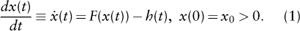
The traditional resource models presented, for example, by Clark (1990) or Dasgupta and Heal (1979) describe the evolution of the population (or biomass or stock) of a biological, a renewable, or an exhaustible resource when exploitation (harvesting) by economic agents takes place. Let x (t) denote the stock of a resource at time t, which generates a flow of valuable services to economic agents. Following the Millennium Ecosystems Assessment (2005) classification, these services may include provisioning services (e.g., food, water, fiber, fuel), regulating services (e.g., climate regulation, disease), cultural services (e.g., spiritual, aesthetic, education), or supporting services (e.g., primary production, soil formation). It should be noted that some of the above services, mainly the provisioning, can be used after harvesting the resources stock (e.g., fishing, water pumping), whereas others, mainly regulating and cultural services, are associated with the existing stock of the resource (e.g., aesthetic services and preservation of a forest). Let F(x(t)) be a function describing the net growth of the resource stock. This growth function embodies factors such as birth, death, migration in case of biological resources (e.g., fisheries), natural inflows, and seepage in case of renewable resources (water resources or accumulation of pollutants), whereas in the case of exhaustible resources with no discoveries, F(x(t)) = 0. If we denote by h(t) the harvesting of the resource, so that provisioning services are used, then the evolution of the resource can be described by an ordinary differential equation (ODE), which can be written, for some initial stock, x 0, as:
The most common specification of the growth function F(x(t)) is the logistic function, F(x)=rx(1 —x/K), where r is a positive constant called intrinsic growth rate, and K is the carrying capacity of the environment, which depends on factors such as resource availability or environmental pollution. If h(t) = F(x(t)), then the population remains constant because harvesting is the same as the population’s net growth. This harvesting rate corresponds to sustainable yield. Harvesting rate is usually modeled as population dependent or h = qEx where q is a positive constant, referred to as a catchability coefficient in fishery models, and E is harvesting effort. The activities of economic agents can affect the resource stock, in addition to harvesting, by affecting parameters such as the intrinsic growth rates or the carrying capacity. Assume, for example, that the intrinsic rate of growth and the carrying capacity of the environment for the resource described by equation 1 are affected by the stock of environmental pollution that accumulates on the ecosystem (e.g., a lake). Let S(t) 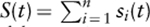 denote the sum of emissions generated by i = 1,..., n sources at time t, and let P (t) be the stock of the pollutant accumulated in the ecosystem (e.g., phosphorus accumulation from agricultural leaching). Then the evolution of the pollutant stock can also be described by an ODE:

where b > 0 is a constant reflecting the environment’s self-cleaning capacity. The negative impact of the pollutant’s stock on the intrinsic growth rate and the environment’s carrying capacity can be captured by functions r (P), r′(P) < 0 and K(P), K′(P) < 0. Then the evolution of the resource is described by:
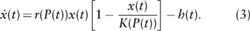
The ODE system (equations 2 and 3) is an example of a simple ecosystem model in which economic agents affect the resource stock in two ways, through harvesting and through emissions generated by their economic activities. The agents that harvest the resource and the agents that generate emissions are, in the majority of the cases, not the same, and it is hard to coordinate their decisions. Furthermore, the pollutant can generate additional environmental damages to individuals, which can be summarized in a damage function.
The simple model of resource dynamics described by equation 1 can be generalized in many ways (see, e.g., Murray, 2003). Generalizations may include age-structured populations, multispecies populations and Lotka-Volterra predator-prey models, mechanistic resource-based models of species competition, models with spatial variation including metapopulation models, and models with resource diffusion over space.
A general multispecies model with J prey populations denoted by xj(t) and J predator populations denoted by yj(i) can be written, for j = 1,..., J, as:
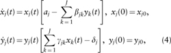
where all parameters are positive constants.
In the mechanistic resource-based models of species competition emerging from the work of Tilman (e.g., Tillman, 1982), species compete for limiting resources. In these models, the growth of a species depends on the limiting resource, and interactions among species take place through the species’ effects on the limiting resource. Let x(t) = (x1(t),xj (t)) be the vector of species biomasses, and R(t) the amount of the available limiting resource. Then a mechanistic resource-based model with a single limiting factor in a given area can be described by the following equations:
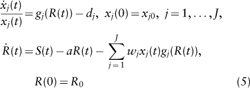
where gj (R) is resource-related growth for species j, dj is the species’ natural death rate, S(t) is the amount of resource supplied, a is the natural resource removal rate (leaching rate), and wj is the specific resource consumption by species j.
Another important characteristic of ecosystems, in addition to the temporal variation captured by the models described above, is that of spatial variation. Biological resources tend to disperse in space under forces promoting “spreading” or “concentrating.” These processes, along with intra- and interspecies interactions, induce the formation of spatial patterns for species in a given spatial domain. A central concept in modeling the dispersal of biological resources is that of diffusion. Biological diffusion when coupled with population growth equations leads to general reaction-diffusion systems (e.g., Okubo and Levin, 2001; Murray, 2003). When only one species is examined, the coupling of classical diffusion with a logistic growth function leads to the so-called Fisher-Kolmogorov equation, which can be written as
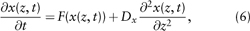
where x(z, t) denotes the concentration of the biomass at spatial point z at time t. The biomass grows according to a standard growth function F(x) but also disperses in space with a constant diffusion coefficient Dx. In general, a diffusion process in an ecosystem tends to produce a uniform population density, that is, spatial homogeneity. However, under certain conditions reaction-diffusion systems can generate spatially heterogeneous patterns. This is the so-called Turing mechanism for generating diffusion instability.
Spatial variations in ecological systems can also be analyzed in terms of metapopulation models. A meta-population is a set of local populations occupying isolated patches, which are connected by migrating individuals. Metapopulation dynamics can be developed for single or many species. For the single species occupying a spatial domain consisting of s =1, ... , S patches, the dynamics becomes
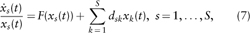
where xs (t) is the species population in patch s, and dsk is the rate of movement from patch k to patch s, (s = k). Thus, dynamics is local with the exception of movements from one patch to the other.
If harvesting is introduced into the ecological models of equations 4-7, and growth functions depend on pollutants generated by economic activities, then the ecological model is extended to include economic variables whose time paths are chosen by economic agents.
Choosing time paths for harvesting or other variables that might affect the state of the ecosystem, which are called control variables, implies management of the ecosystem. In economics, the most common type of management is the optimal management, which means that the control variables are chosen so that an objective function is optimized (maximized or minimized). Of course, other types of management rules can be applied such as adaptive rules or imitation rules, but the focus of the present article is on optimal rules. To provide a meaningful presentation of the optimal rules, some fundamental economic concepts are useful.
Preferences, Utility, Profits
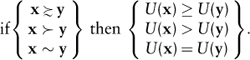
Individuals have preferences summarized by the preference relationship, which means “at least as good as.” Let n goods be indexed by i = 1, ..., n, and the combinations of different quantities from these goods x =(x1,...,xn), y=(y1,..., yn). Then a consumer’s preferences regarding the two combinations or bundles of goods could be described as:
x ≥ y means that combination x is at least as good as combination y.
x > y means that combination x is better than (is preferred to) combination y.
x ∼ y means that the consumer is indifferent between x and y.
A utility function is a real-valued function of the combinations of goods, such as:
A central paradigm of modern economic theory (e.g., Mass Colell et al., 1995) is that, for exogenously determined prices and income, consumers choose the combinations of goods they consume by maximizing their utility function subject to a budget constraint, whereas competitive firms, for exogenously determined prices of inputs and outputs, maximize profits subject to the constraints imposed by technology, which are usually summarized by a production function.
Pareto Efficiency
Economic Allocation
Consider an economy consisting of i = 1, ..., I consumers, j = 1, ..., J firms, and l = 1, ..., L goods. The consumption for individual i is given by the vector xi =(x1i, ..., xLi), and production by firm j is given by the vector yi= (y1j,..., xLj). Consumers maximize profits subject to their budget constraint, whereas firms maximize profits subject to technology.
An economic allocation (x1..., xI, y1,..., yJ)is a specification of a consumption vector for each consumer and a production vector for each firm. The allocation is feasible if
Pareto Optimality
A feasible allocation (x1,..., xI, y1..., yj)is Pareto optimal or Pareto efficient, if there is no other allocation (x′1,..., x′I, y′1,..., y′J)such that u (x′i) ≥ u (xi), ∀i = 1,..., I and u(x′i)> u(xi) for some i. To put it differently, a feasible allocation (x1,..., xI, y1, ..., yJ) is Pareto optimal or Pareto efficient if society’s resources and technological possibilities have been used in such a way that there is no alternative way to organize production and distribution that makes some consumers better off without making someone worse off.
Competitive Equilibrium
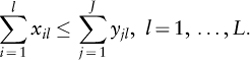
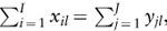
An allocation (x1*,... xI*, y1*,...yJ*) and a price vector p*=(p1*, ..., pL*) comprise a competitive or Walrasian equilibrium if
 l = 1,..., L.
First Welfare Theorem
If the price vector p* and the allocation (x1*,..., xI*, y1*,...yj*) constitute a competitive equilibrium, then this allocation is Pareto optimal.
Second Welfare Theorem
Suppose that (x1*,..., xI*, y1*,..., yj*) is a Pareto efficient allocation, then there is a price vector p*, such that (x1*,...xI*, y1*,..., yj*)and p* constitute a competitive equilibrium.
Welfare Efficiency
A Pareto efficient allocation maximizes a linear social welfare function of the form W =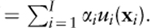
Externalities
Environmental and resource economics have long been associated with the concepts of externalities and market failure. An externality is present when the well-being (utility) of an individual or the production possibilities of a firm are directly affected by the actions of another agent in the economy. When externalities are present, the competitive equilibrium is not Pareto optimal.
Public Goods (Bads)
A public good is a commodity for which use of one unit of the good by one agent does not preclude its use by other agents. Public goods (bads) are not depletable. Environmental externalities (air pollution, water pollution) are nondepletable public bads and are mainly associated with missing markets or missing property rights. Competitive markets have the following characteristics in the presence of externalities:
Economic Policy
The above results imply that competitive markets fail to produce a Pareto optimal outcome or a socially optimal outcome in the presence of environmental externalities and open-access resources. When competitive markets fail to produce the Pareto optimal allocation, there is a need for market intervention and economic policy to achieve the Pareto optimal allocation. Because environmental externalities and open-access characteristics are predominant in ecosystems, competitive (and of course imperfectly competitive) markets fail to attain the socially optimal ecosystem state. Thus, there is a need for economic policy for ecosystem management.
The economic concepts defined above can help formulate optimal ecosystem management and methods for designing economic policy to achieve a socially optimal state for ecosystems. The approach is to define an objective function for the economic agent(s), that will be optimized subject to the constraints imposed by the ecological model of the ecosystem, which will be along the lines of models described in section 2. In principle the objective function will include profits associated with harvesting or utility associated with the ecosystem services. The way in which the objective function is set up, the ecological constraints that are taken into account, determine the solution of the ecological-economic model. By solution we mean the paths for the control variables and the stock of ecosystems resources, which are the state variables, and the equilibrium state of the ecosystem under a specific management rule. Two types of solution are distinguished in general, a socially optimal solution and a privately optimal solution.
The Socially Optimal Solution
The socially optimal solution corresponds to a solution in which social welfare is maximized. This means that the objective function includes utility accruing from harvesting (which is sometimes called consumptive utility and is mainly associated with provisioning ecosystem services) and utility associated with the other services such as regulation, cultural or supporting services, existence values, or benefits associated with productivity or insurance gains (which is sometimes called nonconsumptive utility). The objective function for the social welfare maximization problem also includes damages from environmental degradation, which are environmental externalities (nondepletable public bads), as well as stock effects that negatively affect production functions in the case of management of open access resources. The socially optimal solution is sometimes referred to as the so-called problem of the social planner, where a fictitious social planner maximizes social welfare by taking into account all the externalities not accounted for by competitive markets.
Let Uc (h(t)) denote consumptive utility at time t associated with harvesting h=(h1, ..., hn) species, and Unc (x(t)) denote nonconsumptive utility associated with ecosystem services generated by species biomasses existing in the ecosystem and not removed by harvesting. The total flow of utility at time t can be written as Uc (h(t))+Unc (x(t)). Because the objective in the dynamic context is, in the majority of cases, to maximize the present value of the utility flow over an infinite time horizon, the objective can then be written as:

where ρ ≥ 0 is a utility discount rate, subject to the constraints imposed by the structure of the ecosystem. A solution to this problem will produce the socially optimal paths for the controls and the states (h*(t), x *(t)) and a long-run equilibrium state (h*, x*) as t →∞, provided that the solution satisfies appropriate stability properties. It should be noted that, in principle, benefits associated with consumptive utilities can be approximated using market data from concepts such as consumer and producer surplus, whereas benefits associated with nonconsumptive utility and environmental externalities are hard to estimate because markets for the larger part of the spectrum of ecosystem services and environmental pollution are missing.
The Privately Optimal Solution
The privately optimal solution is distinguished from the socially optimal one by the fact that only consumptive utilities or profits enter the objective function. In particular, when the market outcome regarding the ecosystem’s state is analyzed, the basic assumption is that management is carried out by a “small” profit-maximizing private agent that in general ignores “stock effects,” the general nonconsumptive flows of ecosystem services, or other externalities generated by the agent’s activities. Thus, the private agents do not take into account, or do not internalize, externalities associated with their management. There are some very well-known examples.
In the case of an open-access commercial fishery, usually each harvester takes the landing price as fixed but ignores the fact that his/her own harvesting reduces the stock of fish and thus increases costs. Because the resource has open-access characteristics, each harvester enters in competition to catch the fish first before someone else does. As a result, in the open-access or bionomic equilibrium, the stock of fish is smaller relative to the social optimum, which internalizes “stock effects.” Overfishing and stock collapse can be attributed to this type of externality, also known as the tragedy of the commons. In the case of pollution control, emissions are generated by a group of agents (e.g., an industry), but the damages affect another group of agents (e.g., inhabitants of a certain area). Because the cost of emissions is not internalized by the emitters, in the absence of regulation, emissions exceed the socially desirable level, which is determined by internalizing environmental damages. In other cases harvesters do not take into account nonconsumptive utility associated with the stock of the harvested resource (e.g., existence values), which increases even more the deviation between the social and the private optimum that results from open access. There are also situations in which the harvester does not take into account the fact that harvesting the specific resource might harm the stock of other resources (e.g., by-catch in fishing), which is an additional externality. Another type of externality can be associated with strategic behavior in resource harvesting if more than one economic agent harvests the resource. If many small harvesters are present, then the privately optimal solution can be obtained as an open loop or feedback Nash equilibrium, which also deviates from the social optimum.
The fact that general “stock effects” are not taken into account at the private optimum implies that Unc (x(t)) =0 in equation 8. As a result, the privately optimal solution will deviate from the socially optimal solution. Furthermore, because all the ecological constraints are operating in the real ecosystem, there will be discrepancies between the perceived evolution of ecosystems under management that ignores certain constraints and the actual evolution of the ecosystem. These discrepancies might be a cause for surprises in ecosystem management.
The inability of privately optimal solutions realized in the context of unregulated market economies to attain the socially optimal outcome regarding the state of an ecosystem calls for environmental policy (detailed analysis can be found in Baumol and Oates, 1988; Xepapadeas, 1997), which is assumed to be designed and implemented by a regulator. The classic instruments of environmental policy can be divided into two broad categories.
–Emissions taxes (tax payments related to measured or estimated emissions).
–Landing fees (tax related to the amount of harvested resource from an ecosystem).
–Product charges (consumption taxes, input taxes, or production taxes, which are substitutes for emission taxes when emissions are not directly measurable or estimable).
–Tax differentiation (variation of existing indirect taxes in favor of clean products or activities that are environmentally and ecologically friendly).
–User charges (payments related to environmental service delivered).
–Tax reliefs (tax provisions to encourage environmentally or ecologically friendly behavior).
–Negotiated agreements imply a bargaining process between the regulatory body and an economic agent to jointly set the environmental goal and the means of achieving it.
–Unilateral agreements are environmental improvement programs prepared and voluntarily adopted by economic agents themselves.
–Public voluntary agreements are environmental programs developed by a regulatory body, and economic agents can only agree to adopt them or not.
In general, participation in a VA program exempts the economic agent from stricter regulation.
This type of regulation includes the use of limits on inputs, outputs, or technology at the firm level. When the objective of direct regulation is the firm’s harvesting (e.g., harvesting rates, harvesting periods, “no-take” reserve areas) or emissions, then the type of regulation is called a performance standard. When the regulator requires the use of a specific technology, then the regulation is called a design standard. Performance standards can be associated with a maximum allowed amount of emissions or harvesting, whereas design standards can be associated with the use of best available technologies.
The above classification is by no means exhaustive, and it should be noted that instruments can be used in combinations and that they can be characterized by spatial and temporal variation.
Optimal environmental policy can be designed by using the following approach:
The following example from the literature of determining optimal emission taxation can help clarify this approach. We choose the emission problem instead of an ecosystem management problem because the latter requires the use of more complicated optimal control techniques.
We start by considering a market of i=1, ..., n firms that behave competitively. The firms produce a homogeneous output qi and, during production, generate emissions ei. A derived profit or derived benefit function can be defined as:
where p is the exogenously determined output price, and ci(qi, ei) is a convex cost function decreasing in ei.A reduction in emissions will increase costs because this involves the use of resources for pollution abatement.
Social welfare is defined as total benefits from production less social damages from emissions. Using the derived profit function (equation 9) and a social damage function D(E) which is an increasing and convex function reflecting environmental damages caused by emissions, the social planner solves the problem:

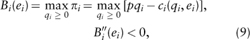
The necessary and sufficient first-order conditions for the socially optimal emissions ei* generated by the i th firm are:

Thus, when positive emissions are generated, marginal benefits equal marginal social damages. The polluting firms fully internalize external social damages if they are confronted with an emission tax per unit of waste released in the ambient environment equal to marginal social damages. This price incentive for emission control is the well-known “Pigouvian tax” or emission tax.
Let the emission tax τ be defined as. 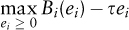 The firm solves the problem

with necessary and sufficient first-order conditions:

Because  it can be seen by comparing equation 11 to equation 12 that the emission tax leads to the socially optimal emissions for firm i, for all i.
In many cases the design and/or the implementation of optimal policy might not be possible because of informational constraints, cost of implementation, and so on. In this case, another approach is for the regulator to set a given standard, such as ambient pollution standards, maximum harvesting rates, minimum safety margins for species populations, and then choose the instrument or the menu of instruments from those described above to achieve the standard at a minimum cost. The policy instruments can be revised or updated as the state of the ecosystem changes or as more information is acquired about the responses of the economic agents and the ecosystem to economic policy. This type of policy is not optimal, but if it is combined with the general insights obtained by having determined the structure of the optimal policy, it might be a useful approach to policy design and implementation.
Baumol, W. J., and W. E. Oates. 1988. The Theory of Environmental Policy, 2nd ed. Cambridge, UK: Cambridge University Press.
Clark, C. 1990. Mathematical Bioeconomics: The Optimal Management of Renewable Resources, 2nd ed. New York: Wiley.
Dasgupta, P. S., and G. M. Heal. 1979. Economic Theory and Exhaustible Resources. Oxford: James Nisbet and Co. and Cambridge University Press.
Mas-Colell, A., M. D. Whinston, and G. R. Green. 1995. Microeconomic Theory. New York: Oxford University Press.
Millennium Ecosystem Assessment. 2005. Ecosystems and Human Well-Being: Synthesis. Washington, DC: Island Press.
Murray, J. D. 2003. Mathematical Biology. Berlin: Springer-Verlag.
Okubo, A., and S. Levin, eds. 2001. Diffusion and Ecological Problems: Modern Perspectives, 2nd ed. Berlin: Springer.
Tilman, D. 1982. Resource Competition and Community Structure. Princeton, NJ: Princeton University Press.
Xepapadeas, A. 1997. Advanced Principles in Environmental Policy. Aldershot: Edward Elgar.