

 |  |


As we’ve just seen, statistical correlations look at relationships when both variables are continuous. When one of the variables is labelled in categories, then we are dealing with statistical associations, specifically the measurement of a variable within categories.
Let’s have a look at an example from Charles Darwin. In 1876, he studied the growth of corn seedlings. In one group, he had 15 seedlings that were cross-pollinated, and in the other, he had 15 that were self-pollinated. After a fixed period, he recorded the final heights of each of the plants.
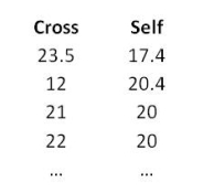
Notice that these data look very similar to the correlations data that we saw in the previous section. They appear to be two columns of continuous data, but it’s just the way they are arranged. We could instead have arranged them as a single column of continuous data with a column labelling the pollination method for each seedling, like this:
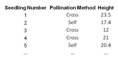
To analyse these data you pool together the heights of all those plants that were cross-pollinated, work out the average height (the arithmetic mean) and compare this with the average height of those that were self-pollinated. You can display the results as a Histogram, like this:
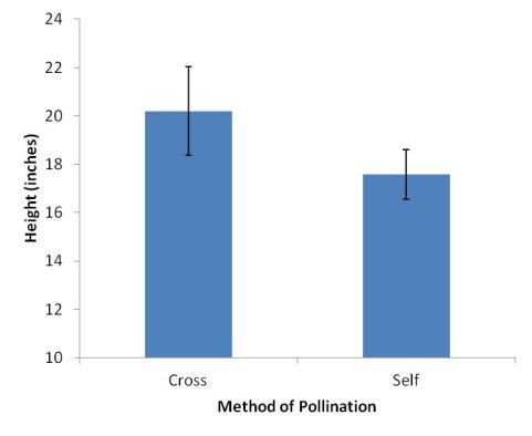
Histogram Showing the Mean Height of Darwin’s Cross-Pollinated and Self-Pollinated Seedlings. Variation is shown by 95% Confidence Intervals.
Darwin found that the average height of the cross-pollinated plants was 20.19 inches, and 17.59 inches for the self-pollinated plants.
Of course, none of the plants were exactly 20.19 and 17.59 inches tall, there was a certain amount of variation in their heights. This variation can be expressed by the standard deviation, variance or other appropriate measure, like the 95% confidence intervals shown.
Scientists tend to use standard deviations to show variation in measurements, but I prefer to use 95% confidence intervals because 95% confidence intervals are related to the statistical tests that you use to decide whether there is likely to be a statistically significant difference between the measurements, so you can usually assess by eye whether there might be a difference.
Quite often, if there is a clear separation between the confidence intervals (in other words, little or no cross over between them) then there is likely to be a statistically significant difference between the groups of measurements.
By eye, there is a clear difference in the heights of the seedlings, and there is no cross over between the pairs of confidence intervals, so there is likely to be a significant difference between the heights of cross- and self-pollinated corn seedlings. We can’t just check by eye, though, we also need to use a statistical test to tell us whether there is a statistically significant difference between the heights of the cross-pollinated and self-pollinated plants. Here, we can use either the 2-sample t-test or the Mann-Whitney U-test.
The 2-sample t-test is used to test whether the means of two groups are the same, and assumes that the mean is the most appropriate measure of centrality for both groups of data. The 2-sample t-test is a more powerful test than the Mann-Whitney U-test as long as this assumption is not violated. The Mann-Whitney U-test, on the other hand, is used to test whether the medians of two groups are the same, and is used as an alternative to the 2-sample t-test when the mean is not the most appropriate measure of centrality for at least one of the groups of data.
So how do we know when the mean is appropriate to measure the centre point of the data?
For this, we need to run a test of Normality. There are a few of these, but we’re going to use the Anderson-Darling test of Normality. If both groups of data pass this test, then we can safely quote the mean as being an appropriate measure of the central point of the data and use the 2-sample t-test to see if there is a statistically significant difference between the heights of the cross-pollinated and self-pollinated plants. If one or both groups of data fail this test, then we should quote the median and use the Mann-Whitney U-test to see if there is a significant difference in seedling heights.
Here is a probability plot, also known as a Q-Q plot, accompanied by the results of an Anderson-Darling test of Normality for the cross-pollination data:
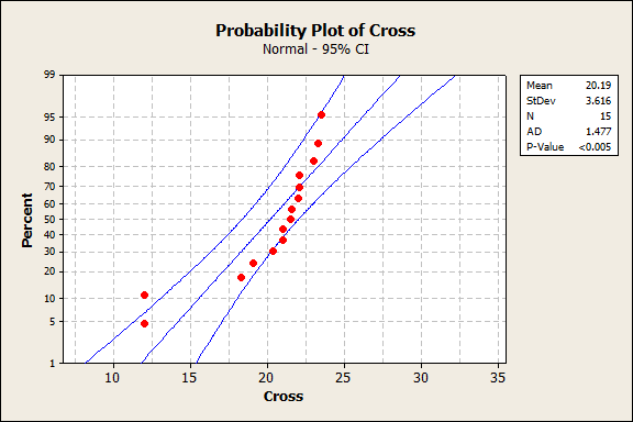
Probability Plot of Darwin’s Cross-Pollination Corn Seedlings
The first thing to check is whether the plot points fall on a straight line (or nearly). They don’t appear to, so these data may not be Normally distributed and we need to check the test p-value. If the p-value is large (>0.05) then the distribution is Normal and the mean is the appropriate measure of centrality. Here, p < 0.05, so we can be sure that the distribution is not Normal, we should not use the 2-sample t-test, but instead use the Mann-Whitney U-test.
The Mann-Whitney U-test orders all the observations from smallest to largest and then ranks them from 1 to N. In this way, the ranks can be compared across the two groups and the actual observations themselves are of no importance, so it doesn’t matter that the data are non-Normal.
Here are the results of the Mann-Whitney U-test for the cross- and self-pollinated seedlings:
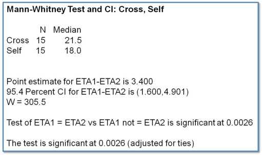
The first thing to notice is that the medians are quoted rather than the means. Next, there are things called Eta 1 and Eta 2. These are the median values of each of the groups, and we are interested in the difference between them, which is 3.4. The 95% confidence interval of this difference is calculated, and what we’re looking for here is whether these confidence intervals straddle zero. If they do, then there is not a significant difference between the medians. In this case, both the upper and lower 95% confidence interval bounds are positive, indicating that there is likely to be a significant difference in seedling heights.
Finally, we check the p-value to see if this is the case. As p < 0.05, we can conclude that Darwin’s cross-pollinated corn seedlings were indeed significantly taller than the self-pollinated seedlings.
That’s not quite the end of the story, though. Remember right at the beginning that we showed a histogram displaying the means and 95% confidence intervals? Well, we’ve just established that these are not appropriate measures to use, and we should instead use medians. When publishing our results, we should then use a Box-and-Whiskers plot, like this:
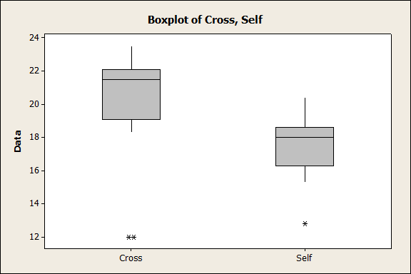
Box-and-Whiskers Plot of Darwin’s Cross-Pollinated and Self-Pollinated Corn Seedlings
In a Box-and-Whiskers plot, the box part is the Inter-Quartile Range (from the 1st quartile to the 3rd quartile of the data), and the bar across the middle is the median. The whiskers protruding out of the top and bottom of the box tell us the limits of our data. That’s not quite the end of it though, because sometimes there are values that fall far outside the quartiles. These are the outliers and are usually plotted as separate points.
OK, so we’ve established that the data are not Normally distributed, so the medians are more appropriate than the means, and the Mann-Whitney U-test is more powerful than the 2-sample t-test for these data. We also discovered that Darwin’s cross-pollinated corn seedlings were significantly taller than his self-pollinated seedlings.
What if, on the other hand, we discovered that the data were Normally distributed? Well, then we can use the 2-sample t-test. Let’s go ahead and do that, just to see where it takes us:
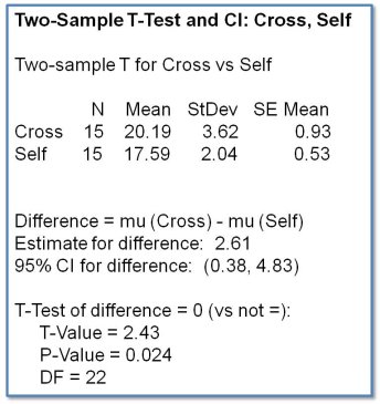
Here, the means are quoted along with the standard deviation and the standard error of the mean. We’re interested in the difference between the means, which is 2.61. The 95% confidence interval of this difference is calculated, and, as with the Mann-Whitney U-test, what we’re looking for here is whether these confidence intervals straddle zero. Again, both confidence interval bounds are positive, and the p-value is significant, telling us that the cross-pollinated corn seedlings were significantly taller than the self-pollinated seedlings.
So, for these data it didn’t matter whether we chose the most appropriate statistical test (the Mann-Whitney U-test) or the alternative (the 2-sample t-test). Both gave us the same result.
That doesn’t mean that we can be complacent though. We must still endeavour to choose wisely, as this might not always be the case, and making a poor choice of statistical test could give us an incorrect result.
Now I don’t want to come off as being some kind of a pest. I don’t want you to think I’m any kind of a pest, but I bet you haven’t visited the Resources page yet have you? Hands up if you haven’t visited yet...
When you get to the end of this book, you’ll read my bio, and when you do, you’ll discover that my mission is to unleash your inner data ninja.
It wouldn’t be much of a mission if I couldn’t get you to visit one little blog post where you can find all the resources you’ll need to learn about associations and correlations, would it?
Don’t forget, there’s all sorts of FREE stuff there for you to find, so pop on over – I’ll see you when you get there: