Comparing Sample and Remote-Sensing Data—Understanding Surface Composition
Abstract
Almost everything done in planetary science and astronomy could be considered “remote sensing.” For almost all of our investigations, photons are emitted or reflected from a surface, however close or far, and then it comes to us carrying information about that surface. How we collect and analyze that light is the key to understanding the surface. However, there is a substantial difference in understanding surfaces that we cannot physically touch or interact with, and those we can. Objects that are far away, and that are viewed only with telescopes or spacecraft are targets for “remote sensing.” Objects that we have in hand, and that we can study on Earth with laboratory equipment are subject to “sample analysis.” Of course, these general definitions are not black and white. With the advent of remote laboratories, such as a string of sample handling and analyzing landers and rovers on Mars, what is considered “remote” and what is considered “in hand” can become blurred. The bringing together of sample and remote-sensing data has reaped great rewards in planetary science. We use the samples we have, whether returned by spacecraft or brought to us by nature, to do in-depth laboratory studies. These studies can be tied to remote-sensing techniques, which let us extend what we have learned to areas or objects for which we have no samples. As laboratory and remote-sensing data become more detailed, what we learn from each technique helps us better interpret data from other techniques.
Keywords
Remote sensing; Data; Craters; Meteorites; Asteroid; In situ; Laboratory studies
The Importance of Comparing Data Sets
Almost everything done in planetary science and astronomy could be considered “remote sensing.” For almost all of our investigations, photons are emitted or reflected from a surface, however close or far, and then it comes to us carrying information about that surface. How we collect and analyze that light is the key to understanding the surface. However, there is a substantial difference in understanding surfaces that we cannot physically touch or interact with, and those we can. Objects that are far away, and that are viewed only with telescopes or spacecraft are targets for “remote sensing.” Objects that we have in hand, and that we can study on Earth with laboratory equipment are subject to “sample analysis.” Of course, these general definitions are not black and white. With the advent of remote laboratories, such as a string of sample handling and analyzing landers and rovers on Mars, what is considered “remote” and what is considered “in hand” can become blurred.
Given that so much of planetary science and astronomy requires light from remote sources, it is critical that we understand the collection and analysis of such light as well as we can. An integral part of this picture is comparing remote-sensing data to data collected in the laboratory whenever possible. In the lab, we have the luxury of conducting many different kinds of tests on samples that are not (yet) possible to conduct remotely. For example, to study a lunar rock from the Apollo collection, one might make a thin section of the rock, and then place it in a petrographic microscope for inspection. We do not have the means to create thin sections on rovers at this time, so this kind of analysis can only be done on laboratory samples we have here on Earth. By performing “ground truth” on our remote measurements by using sample analysis, we enable better, more appropriate use of remote measurements and extend what we have learned in the laboratories beyond what we have already sampled.
It is only in understanding what we have in hand that allows us to construct a picture using remote-sensing data. And of course our starting point, both historically and in scientific investigations, is looking at the world close around us, and then extrapolating outwards.
Terrestrial Analogs
The starting place for understanding airless bodies, or indeed any astronomical body or phenomenon, is the planet right at our feet. Although the Earth does have an atmosphere, and is subject to many surface processes one does not find on airless bodies, it still forms our first step in understanding. It is here we can closely observe, and closely sample, the rocks and features of the biggest of the four terrestrial planets. Comparing sample and remote-sensing data from Earth to other planets allows us to make both basic and subtle interpretations of what we are seeing.
One glance at the Moon shows a major surface dichotomy—bright terrain and dark terrain. On closer examination, one sees that the bright terrain is topographically higher and rougher than the flat, low-lying dark terrain. Speculation about what this dark terrain might be has been the purview of countless generations, giving rise to the name “mare,” Latin for “sea.” Examination with telescopes (and more) along with comparison with terrestrial analogs gave us a much more accurate idea of what these areas might be.
Flood basalts, one of the most common terrains on Earth, are areas where vast amounts of lava have flowed over the surface and subsequently hardened. Visiting the Moon and bringing back samples of rock confirmed that the mare are indeed vast plains of volcanic rock. Indeed, flood basalts are one of the most ubiquitous features on the terrestrial planets (Fig. 5.1).

Interpreting Craters
One example of the power of comparing sample data to remotely sensed data is that of the final determination of the origin of craters. The first views of the surface of the Moon through telescopes revealed circular surface features of unknown origin. Scientists looked to our own planet to try to understand what they were seeing. On Earth they found similar structures, but of two types—those that were suspected to be of impact origin, and those suspected or known to be of volcanic origin.
Our use of terrestrial analogs for these surface features thus allowed us to produce two schools of thought about these circular lunar features (Fig. 5.2). In the end, the remote-sensing data were inadequate, even with these analogs, to end the debate. In part, confusion over the nature of terrestrial impact craters and the physics involved in their creation didn’t help matters. Based on their everyday experience, scientists who thought lunar craters were primarily volcanic argued that impactors coming from random directions and random angles above the horizon would create elliptical craters, rather than the circular shapes that dominated the lunar crater population. It wasn’t until we actually visited the Moon and brought back samples that it was conclusively decided that the structures were impact craters, not volcanic calderas (Wilhelms, 1993).

Bulk Density: Implications for Surface Composition, Interior Structure, and Volatile Content
Although this book focuses on surface processes, a brief look at the overall density of the terrestrial worlds and certain example asteroids is important to understanding the nature of a body's surface composition. The concept of bulk density and what it can tell us about a body is an important example of how we can compare what we know about samples in hand (rocks and ice) and what we determine by remote means (mass and thus density).
At their most simple, solid planetary bodies are made of three bulk constituents: ice (H2O), rock (SiO2 and related crystals), and iron (metals). Average densities for these materials are 1000 kg/m3 for ice, and approximately 3000 and 8000 kg/m3 for rock and iron. (Note that densities vary depending on conditions.) The basic composition of a body can be estimated by using bulk density, assuming that the body is not substantially porous.
Table 5.1 lists the compressed and uncompressed densities for certain rocky planetary bodies. For worlds with substantial mass, gravity compresses the body such that mineral densities are higher than at standard pressure and temperature. Worlds smaller than the Moon lack enough gravity to compress themselves to any substantial degree.
Table 5.1
| Body | Compressed | Uncompressed |
|---|---|---|
| Mercury | 5400 | 5300 |
| Venus | 5200 | 4000 |
| Earth | 5500 | 4400 |
| Moon | 3400 | 3300 |
| Itokawa | 1900 | 1900 |
| Eros | 2700 | 2700 |
| Mars | 3900 | 3700 |
| Phobos | 1900 | 1900 |
| Deimos | 1500 | 1500 |
| Vesta | 3500 | 3500 |
| Ceres | 2200 | 2200 |
Objects are listed in order of average distance from the Sun.
To compare on the basis of composition, we view the uncompressed column.
For any world massive enough to differentiate, low-density materials are not stable below high-density materials. Differentiation will preferentially allow low-density materials like ice to move to the surface of a body, and will allow high-density materials like iron and nickel to move toward the core. Therefore, the surface composition of a differentiated world (as determined either by sample analysis or remote sensing) along with bulk density provides distinct insight into the overall composition and structure of a world.
For example, choosing only from the three broad categories of bulk constituents, and using surface samples, we classify the Moon's surface as made of rock (3000 kg/m3). With an uncompressed density of 3300 kg/m3, we can infer that the Moon's interior is also largely rock, with the potential for a small iron core. The Earth's uncompressed density is 4400 kg/m3, and its rocky surface therefore suggests a more substantial iron core.
When ice is a suspected constituent, the implications for volatiles and interior structure become obvious. Note Phobos and Deimos, with bulk densities of 1900 and 1500 kg/m3, respectively. Such low densities might otherwise suggest substantial ice content. However, remote-sensing and modeling data do not suggest ice as the primary surface constituent for these worlds. Instead, it is suspected they are not coherent bodies, but that they possess high porosity on large and small scales, lowering their density dramatically. See discussion in the volatiles chapter for more details.
On the other hand, the densities of Vesta and Ceres do indeed seem consistent with our view of their constituents. Vesta, a differentiated, rocky world, has a density of 3500 kg/m3. Remote-sensing data and sample data in the form of HED meteorites support the idea of a rock surface and a small metallic core. Ceres’ low density as well as telescopic measurements of its hydrated minerals in conjunction with models of its thermal history and formation of those minerals, suggested ice as an important bulk constituent. This has been verified by the findings of the Dawn Mission.
Meteorites
Meteorites are pieces of other worlds that have survived their fall to the surface of the Earth still intact. Although most of the smaller dust-sized material that hits our atmosphere burns up on impact (meteors, i.e., “falling stars”), larger pieces can survive their journey all the way down. The largest pieces will of course form impact craters (Chapter 7). While some meteorites are seen to fall and are collected shortly after arrival (these are fittingly called “falls”), most known meteorites are collected long after they fell (these are called “finds”) and are subject to terrestrial weathering effects (Fig. 5.3). While falls are more pristine, some unique compositions are found among the finds, and a large amount of work has been done to correct or account for the way the finds have been altered.

The worlds from which meteorites are derived can theoretically include any rocky surface, such as the Moon, Mars, and asteroids. We have positively identified meteorites from these places. It is not impossible that we also have pieces of Mercury or Venus on our planet, and have simply not yet found or properly identified them.
Meteorites from places such as the Moon and Mars will include evidence of the history of that body, including its differentiation, volcanism, and more. But for their part, meteorites from asteroids can have very complex histories that are difficult to unravel. Because we usually do not know the particular asteroid that the material came from, we do not have geologic context. Some meteorites, such as the HED meteorites, have been positively identified as being derived from the asteroid Vesta. In this case, we say that Vesta is the parent body. But the parent bodies for other meteorites are not specifically determined, and some of these bodies may well have been completely destroyed by an impact event in the deep past. Even in cases where we can identify the parent body of a meteorite, we can only guess where on that parent body the sample formed.
Meteorite Types—Compositional Classification
The oldest known meteorites were formed during the very earliest days of the solar system. Planetary systems with their central star(s), attendant planets, and belts of material, are formed from collapsing disks of gas and dust. Most of the bulk of the original material in this stellar cloud ends up in stars, or blown out of the systems entirely by stellar winds. But there is plenty of material left over in the systems for the creation of planets and asteroids.
The material that accreted into large bodies such as the Earth, Mercury and the Moon, was altered by the processes on those bodies. For example, for an Earth-like planet, temperatures are high enough that the material making up the planet becomes molten. Denser materials such as Fe and Ni metal sink to the center, while less dense materials bearing Ca and K rise to the top. This process of differentiation dramatically changes the nature of the original material that accreted to form the planet.
While the composition of asteroids and meteorites is the subject of many excellent works and an in-depth discussion is beyond the scope of this book (however, see the Additional Reading at the end of the chapter), it will be helpful to provide a brief overview of the topic since it is a factor in many of the processes we see on small-body surfaces.
The vast majority of meteorites are thought to come from asteroids (the few others are thought to come from Mars and the Moon, the latter group further discussed later). In broad terms, meteorites are divided into two groups: the chondrites and the achondrites (Fig. 5.4). The chondrites are undifferentiated: they contain silicate minerals and iron/nickel metal in close proximity, and geochemical and textural evidence shows they have remained below their melting temperatures since formation. Chondrites are named for chondrules, mm-scale glass spheroids that are ubiquitous in most chondrite groups. Their elemental compositions match the composition of the Sun as derived from astronomical studies, when the difficulty of incorporating noble gases and extremely volatile elements like hydrogen into minerals is factored in. This has in turn been used to identify chondritic meteorites as the likely starting materials for the inner planets.
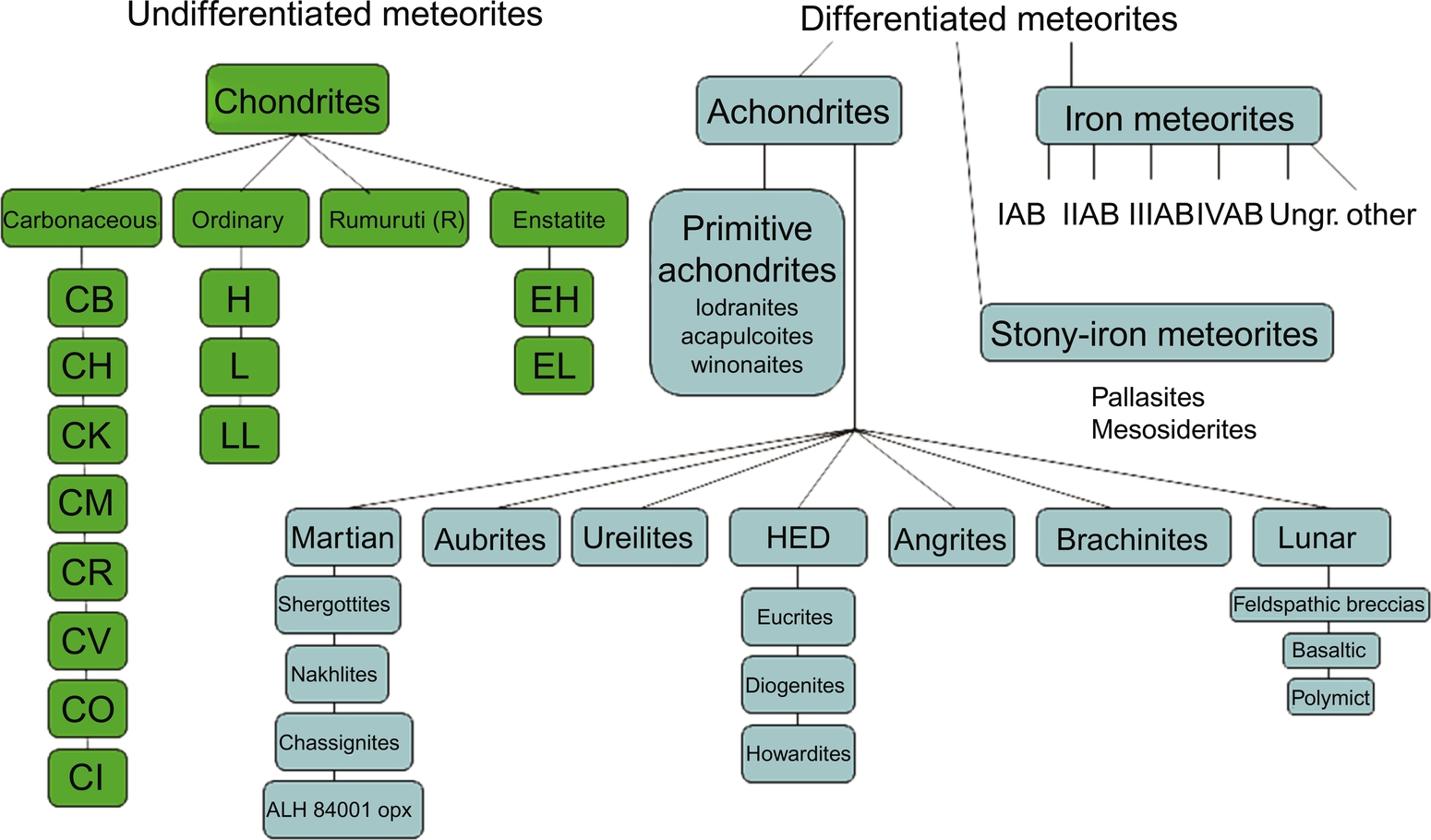
Chondrites are subdivided into 5 groups: C (“carbonaceous”), O (“ordinary”), E (“enstatite”), R, and K. The latter two groups are uncommonly seen, while thousands of C and E chondrites are known and nearly 50,000 O chondrites are known. This classification scheme has roots roughly a century ago, when the preponderance of O chondrites led to them being labeled “ordinary” and other gross observations led to the labeling of the “carbonaceous” and “enstatite” groups. While the descriptive names for the meteorite groups may not be useful at this point (not all C chondrites qualify as particularly “carbonaceous”), these names are still in common use in the community (and occasionally in this book1).
The chondrite groups are distinguished from one another by relative amounts of oxidized and metallic iron, elemental or isotopic ratios that point to different formation conditions, presence or absence of specific minerals, etc. Of the three largest groups, it is generally seen that the E chondrites are least oxidized, followed by the O chondrites and finally the C chondrites. The OC meteorites are divided into the H, L, and LL groups based on their concentration of iron: “high,” “low,” and very low. The C chondrites are commonly seen to have hydrated and hydroxylated minerals indicating aqueous alteration has occurred, though such alteration has not changed the overall elemental balance. A very small number of O chondrites have hydrated minerals. It is thought that at least some C chondrite groups once had hydrated minerals that were then destroyed by later heating. Similarly, there is some evidence that at least some non-C chondrites also once had hydrated minerals that were later destroyed.
Achondrites were first defined simply as meteorites lacking chondrules. There are six main asteroidal achondrite groups, all of which show evidence of igneous processes on a parent body that at least partially differentiated. The most common achondrite group is the HED meteorites (named for three subgroups: the howardites, eucrites, and diogenites), thought to come from the asteroid Vesta. Eucrites are basaltic rocks, diogenites are plutonic (cooled beneath the surface), and howardites are brecciated mixtures of eucrites and diogenites.
The aubrites and angrites represent igneous samples from other parent bodies—the aubrites are also called “enstatite achondrites” and are thought by many to be connected to the E chondrites. The other major groups of achondrites have high concentrations of metal. The iron meteorites are almost entirely composed of iron, nickel, and other elements that geochemically favor incorporation into metallic iron alloys. The mesosiderites are breccias of iron-nickel metal and pyroxene-rich silicates, while pallasites contain olivine and metal and are not brecciated. In both cases, the silicate fraction can vary but is usually several tens of percent. As noted elsewhere, the surface processes on metallic asteroids are very poorly known and are not considered in this book unless specifically mentioned.
Finally, the primitive achondrites are rocks that have experienced some melting (usually a very low degree) but have not experienced differentiation. The origin of the primitive achondrite groups, and which other meteorite groups they are most likely related to, is a matter of ongoing research.
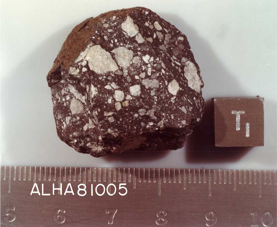
Lunar Meteorites
Although representing a rare fraction of meteorites, lunar meteorites are consistently being recovered from the Earth's hot and cold deserts (Fig. 5.5). These locations allow for the positive identification of these rocks, which may appear terrestrial to the untrained eye. As of this writing, many dozens of lunar meteorites have been collected or identified in meteorite collections. We do not know the specific geologic context for these samples; that is, we do not know from what locations the rocks derive, as each was liberated by a random impact event in an unknown area some time in the past (Korotev, 2005).
Coarse remote sensing of the Moon might suggest two major lithologic provinces; the highlands and the mare. Such a bimodal paradigm of lunar geology has long been held by lunar scientists. This view initially seemed to be borne out by the samples returned by Apollo. These samples included what were thought to be two major geochemical suites, each corresponding to mare or highlands. However, the Apollo missions all landed in the anomalous Procellarum KREEP Terrane, and returned samples enriched in Th. This Th-rich material was dispersed all over the region by one of the last huge basin forming impacts. Without the backup of remote-sensing orbital data (which was not provided until years later), there was no challenge to the standing bimodal paradigm. It is the lunar meteorites that provided, and continue to provide, further insight into the Moon's three geochemically distinct provinces.
Korotev notes three extreme types of compositionally and lithologically distinct lunar meteorites (note, some meteorites fall between these designations, and a few are not represented here):
- (1) Brecciated anorthosites. These have high aluminum, low iron, and little thorium.
- (2) Basalts and brecciated basalts. These have high iron, relatively low aluminum, and moderate levels of thorium.
- (3) Impact-melt breccia of noritic composition, levels of aluminum and iron intermediate to the first two types, and very high thorium. These are similar to the Apollo “KREEP” compositions.
This new view of lunar geochemistry has advanced ideas about the lunar crust and its compositional diversity. This heterogeneity may point to the lunar crust having formed in something other than a single magma ocean event (Joy and Arai, 2013).
An example of the power of comparing sample and remote-sensing data is an attempt to locate the launch locations of the lunar meteorites using orbital lunar geochemistry. Work by Calzada-Diaz et al. (2015) uses the Lunar Prospector gamma ray spectrometer remote-sensing data set for the elements Fe, Ti, and Th as applied to 48 lunar meteorites. They find that basaltic and intermediate Fe regolith breccias have the best constrained potential launch sites. Highland feldspathic meteorites are less well constrained. Constraining the launch locations for the lunar meteorites may improve our understanding of the impact flux, as well as our models of the composition of the lunar crust.
Telling the Story of a Meteorite
Determining the history of a meteorite from its origin on a parent body can be quite complex. In order to begin to create a timeline of events for a meteorite, several research studies must be conducted including petrographic analysis, Argon (or other) age determination, CRE age determination, and the examination of any possible history or eye-witness accounts of the fall and retrieval of the meteorite.
Take, for example, the history of the Cat Mountain meteorite as determined by Kring et al. (1996) and presented in Table 5.2. The Cat Mountain meteorite came from an asteroid that accreted approximately 4.55 Ga ago, based on the presence of chondrules in the sample. After that, there is a record of a thermal impact event on the parent body at 2.7 Ga that likely produced a crater. This we know from degassing in the argon age profile, and from the creation of shock veins in the clastic material.
Table 5.2
| Time of event | Nature of event | Evidence for event/how we know |
|---|---|---|
| ~ 4550 Ma | Accretion of parent body | Contains chondrules |
| ~ 2700 Ma | Thermal impact event on parent body, crater | Degassing in argon profile (Ar age) Creation of shock veins in clast material |
| 880 Ma | Major impact event, crater sample buried | Argon degassing, profile age (Ar age) Cooling of material |
| 880–20 Ma | Major impact event, Jettisoned sample | Had to be jettisoned after one impact, and before CRE age |
| 20 Ma | Impact event, m-sized object | CRE age |
| ~ 1980 | Collision with Earth Sample collected | Sample in hand Sample found on path |
| ~ 1990 | Sample identified | Meteorite confirmed |
From Kring, D.A., Swindle, T.D., Britt, D.T., Grier, J.A., 1996. Cat mountain: a meteoritic sample of an impact-melted asteroid regolith. J. Geophys. Res. Planets 101 (E12), 29353–29371.
At approximately 880 Ma, there was a major impact event that probably produced a crater and also buried our meteorite sample. Again, our clue is the degassing event in the argon age profile, and examination of how the material cooled thereafter. Sometime between 800 and 20 Ma, the sample was subject to a major impact event that jettisoned it from the parent body. We know this because we have an age for the 880-Ma impact event, as well as a 20-Ma CRE age, so the sample was jettisoned in between. The CRE age of 20 Ma both gives us a lower bound on the previous event, and suggests an impact event on that jettisoned material that reduced it to a meter-sized object.
In approximately 1980, the sample collided with the Earth, and the sample was collected. We know this because we have the sample in hand—it was found on a path in the Arizona desert near Cat Mountain. It remained in a desk for approximately 10 years, and then was finally identified as a meteorite in approximately 1990.
This example makes it clear that creating a timeline of events for a piece of an asteroid can be a complex endeavor. Multiple research and study approaches are necessary. And still, the particular parent body has not been identified, assuming it still even exists. Nevertheless, a great deal of the history of this rock can be determined, and in concert with similar studies of other samples and additional remote sensing, we can piece together an overall history of the solar system.
Interplanetary Dust Particles
Below sizes of mm-cm, extraterrestrial impactors take on a different character than meteorites and are classified separately. Interplanetary dust particles (IDPs) are ~ 5–25 μm in diameter, and are collected by high-altitude aircraft: the only natural terrestrial sources of IDP-sized particles in the stratosphere are volcanic eruptions, with human-made materials like aircraft or rocket exhaust and particles lofted by above-ground nuclear tests serving as the only other sources of material. IDPs are easily distinguished from such particles. Micrometeorites (MMs) are larger (up to hundreds of μm in size) and tend to be collected from polar ice or Antarctic wells. It is thought that IDPs come from both asteroidal and cometary sources, but the relative importance of each source is still a matter of ongoing research and debate. Recent family formation events in the main belt are the sources of most asteroidal dust, while emission from a large number of individual comets during volatile sublimation provides the cometary contribution. The dynamics and nongravitational forces on IDPs and MMs are discussed further in Chapter 9.
Compositionally, there are two types of IDPs: nonchondritic and chondritic. The first group is often simply single mineral grains, with masses of order nanograms. Studies suggest that as much as 10 g from an asteroid is needed to obtain a representative sample, so deviation of such a small mass from chondritic elemental ratios does not necessarily mean it originated on an achondrite. Chondritic particles dominate the IDP collection and are generally divided into three compositional groups: pyroxene, olivine, and layer silicate. Given the logic stated for the nonchondritic IDPs, it is a surprise that particles this small have chondritic ratios, and it demonstrates that IDPs are not simply small fragments of known meteorites. Indeed, many of them are agglomerations of mineral grains with particles sizes < 5 μm. The composition of the layer silicate (also called “hydrated”) IDPs shows that these objects experienced aqueous alteration on a parent body, thought to be asteroids rather than comets. Vernazza et al. (2015) used this argument in part to conclude that IDPs originated on large C-complex asteroids like Ceres, which appear to be underrepresented (or in some cases absent) in the C chondrite collection.
Sample Collection Missions
Robotic spacecraft missions that have collected actual samples of material are few and far between. In spite of the tremendous scientific value of pristine samples, and of those with established geologic context, such missions are both expensive and often deemed high risk. In-depth details about these missions can be found on websites listed in the Additional Reading section at the end of this chapter, but here we summarize basic information about nonlunar missions.
Stardust
The NASA Stardust mission was designed to be the first mission that would return samples from a comet. In addition, it was designed to collect samples from interstellar space that constantly stream through the Solar System. After its launch in February of 1999, the spacecraft encountered comet 81P/Wild (then named “Wild 2”) in January of 2004. In order to collect samples of the comet, the spacecraft was sent through the comet's coma. Dust grains from the comet were entrained in a specially designed collector composed of silica aerogel that was exposed during the flyby. The sample tray was then closed to keep the samples pristine. A capsule with the samples onboard was sent back to the Earth, where it came down in January of 2006 (Fig. 5.6). The samples were taken to the dedicated Stardust Laboratory at the Johnson Space Center. Upon analysis, they showed that there was a great deal more mixing between inner and outer solar system materials than was previously hypothesized. One technical finding of the mission was that aerogel was not the material best suited for collection of fragile materials. The Stardust mission was equipped with a camera that did characterization of the comet nucleus. After the sample was jettisoned, the primary spacecraft went on to encounter another comet (9P/Tempel aka “Tempel 1”), which was the target of another mission, Deep Impact.

Hayabusa
The first sample return mission for JAXA (The Japanese Aerospace Exploration Agency) was Hayabusa. The mission was designed to collect several grams of material from the asteroid Itokawa. Launched in May of 2003, Hayabusa encountered Itokawa after a 2.5-year cruise.
Asteroids have such low gravity that the methods of sample collection must of necessity be quite different from those used on planets. A standard “scoop” method for example might push the spacecraft over, or even right off of the asteroid. Instead the spacecraft lightly encounters or even softly bounces in a controlled fashion, and collects samples through various means on each bounce, a technique called “touch and go” or TAG sampling. Hayabusa was designed to fire a pellet to dislodge surface samples upon contact, with contact during each bounce to last a few seconds—not very long, but long enough to collect samples. A series of mishaps complicated the process, and it was discovered that the pellet did not fire. It was also discovered that during one landing attempt, the spacecraft unintentionally spent an extended period on Itokawa's surface with its sample canister open to space.
However, in spite of the damage to the spacecraft accrued by these mishaps, it was able to come back to Earth in June of 2010. After retrieving the spacecraft, thousands of tiny (10–100 μm) grains (totaling less than a milligram of mass) were discovered in the sample container, in spite of the fact that the original sampling process did not work. Even though the amount of material is much less than was hoped, the geologic context for the samples is known and well characterized by remote-sensing instruments on Hayabusa, and from the ground. They are the first direct samples of an asteroid that were collected. The gamma ray and X-ray spectrometer, the imaging data, and samples all point together to indicate Itokawa has the same composition as ordinary chondrites (Nakamura et al., 2011).
Genesis
Launched in August of 2001, the Genesis mission was designed to collect solar wind particles in order to better determine the composition of the Sun. The composition of the Sun is important to planetary science because it represents the general composition of the original solar nebula from which all the planets accreted. The spacecraft remained at the L1 Lagrange point between the Earth and Sun for 2 years and 4 months. It eventually came back to Earth in 2004; however, it suffered a hard landing because of a parachute failure, leading to concern that the mission would be lost. In spite of this, the samples were retrieved and brought to the laboratory for analysis. The main result from Genesis concerns oxygen isotopes, as it was found that the Sun is more enriched in 16O than rocky solar system bodies. This suggests that 16O was somehow depleted, or other oxygen isotopes enriched, as inner solar system materials were forming (McKeegan et al., 2011)
Morphological Imaging
Photogeology is a long-standing, well-established technique for understanding surfaces. A full discussion of photogeology is well beyond the scope of this book, but we note that these techniques are commonly applied to the airless bodies for the identification of landforms like craters, ridges, lava flows, landslides, etc.
Data for morphological studies are generally taken with cameras very much like the ones in common use by the public. There are two types of camera modes: framing and TDI (“time delay and integration,” commonly called “pushbroom”). Framing cameras take an exposure of a fixed length, with the entire image obtained simultaneously. This is the same way that everyday cameras we use operate. Pushbroom imagers are more like the panorama mode in mobile phones, with the image built up line by line over time. While mobile phone panoramas typically require movement of the camera, spacecraft pushbroom imagers often stare in a fixed direction and build up images from the spacecraft orbital motion around the target. Pushbroom imagers are often imaging spectrometers, returning a full spectrum for each line of spatial coverage resulting in a 3-D image cube with two spatial and one spectral dimension.
Cameras can have very high spatial resolution. The narrow-angle camera (NAC) on LRO returns images at 50 cm/pixel, so a full image will only cover ~ 1 km2. The surface area of the Moon is nearly 38 million square kilometers, so a given NAC frame may not be easy to find on a full map of the Moon. As a result, the LRO NAC is paired with a wide-angle camera (WAC) pointed at the same location as the NAC and providing 100 m/pixel imaging to provide context for the NAC images. This arrangement of a NAC + WAC imaging system is common on planetary missions to larger objects like Mercury. Other objects like Eros and Itokawa are sufficiently small that even very high spatial resolution images capture a significant fraction of their surfaces: a 10-cm pixel scale for an imaging array of 2000 × 2000 pixels would capture well over half of Itokawa in a single image. Because relatively few WAC images are needed to cover an object compared to the number of NAC images, WAC instruments are commonly constructed with color filters and the ability to take spectrophotometric data. Conversely, the high spatial resolution of NACs typically requires them to be taking data at a very high rate while still typically imaging only a relatively small fraction of a target surface.
Asteroid Spectral Classes
The first large asteroid spectral survey was undertaken in the early 1970s using the 0.3–1.1-μm range. By the mid-1970s, the outlines of a taxonomy were being adopted using spectrophotometric data in those wavelengths combined with albedos where available. The major spectral groupings were given single-letter mnemonics meant to broadly associate them with meteorite types: C for carbonaceous, S for “silicaceous” or “stony” (i.e., the OC and achondrites other than iron meteorites), and M (iron meteorites). A formal taxonomy from the mid-1980s (the “Tholen taxonomy” named for its creator: Tholen, 1984) used most of the English alphabet as names for different classes. A spectroscopic survey in the late 1990s led to the establishment of a new taxonomy, the “Bus taxonomy,” intended to be backward compatible with the Tholen taxonomy (Bus and Binzel, 2002). The Bus taxonomy was extended in the last decade to include data to 2.5 μm, and is now called the “Bus-DeMeo taxonomy” after its main authors (DeMeo et al., 2009).
Both the Tholen and Bus-DeMeo taxonomies have particular strengths. The Tholen taxonomy includes albedo, and is able to distinguish between some groups that have similar spectral properties but very different reflectances. It also has a shorter wavelength cutoff than the Bus-DeMeo taxonomy, and several classes are distinguished from one another on the basis of behavior in the 0.35–0.5 μm region. The Bus-DeMeo taxonomy benefits from much higher spectral resolution than the Tholen taxonomy as well as a much longer wavelength cutoff since the 1–2.5 μm region was added. The spectral resolution has allowed the consistent identification of absorption features that have been used to distinguish between classes (Fig. 5.7).

It was noted by Tholen that three classes (the E, M, and P classes) required albedo information to be separated from one another: the E asteroids had very high albedos (> 0.3), the P asteroids low albedo (< 0.08), and the M asteroids had albedos in between. Those asteroids with E/M/P-class colors but no albedo were put into a special “X class” until albedo information was obtained. The Bus-DeMeo taxonomy includes three large, broad “complexes” (C, S, and X) that mirror the C, S, and M classes from the first taxonomies. Because it does not use albedos, members of the E/M/P classes in the Tholen taxonomy are grouped together in the Bus-DeMeo taxonomy. Roughly speaking, the C complex consists of asteroids with relatively flat spectra, the X complex asteroids with somewhat red-sloped spectra (having increasing reflectance with increasing wavelength), and the S complex has objects with 1- and 2-μm absorption bands due to mafic silicates. Within each of these complexes are several classes, which tend to be distinguished from each other by spectral slope differences and the presence/absence of additional absorption bands.
The complementary strengths of the two taxonomies have led to a de facto adoption of a hybrid system by many asteroid scientists. Typically, it uses the Bus-DeMeo classes along with the Tholen E/M/P classes, so one may read about Ch-class asteroids experiencing aqueous alteration while P-class asteroids did not. While this approach makes sense in some situations, it also runs the risk of confusing matters or assuming a one-to-one correspondence between classes in each taxonomy where no such correspondence exists (such as between the Xe and E classes).
In addition to the major C/S/X groupings in these taxonomies, both taxonomies include a number of other classes independent of the broad complexes. These include a V class to hold objects with Vesta-like spectra, a D class for very red objects with comet-like colors, and a T class about which little compositional information is available. Table 5.2 lists some of the more common asteroid spectral classes along with example asteroids and our best understanding of meteorite analogs.
It is worth noting and emphasizing that while asteroid spectral classes are defined by spectral characteristics and those characteristics are related to the asteroid compositions, determining the spectral class of an asteroid is typically not sufficient to determine its composition. This is particularly true of those spectral classes that are generally featureless in the 0.4–2.5 μm region and differ only in spectral slope. It is also worth noting that asteroid spectral surveys typically visit each target only once. Because spectral slopes are a function of phase angle, the spectral class for some featureless asteroids could be affected by the geometry at the time of observation, and additional observations might place them in a different class. As a result of all of this, asteroid spectral classes are best considered to be gross indicators of composition and best suited for statistical studies of differences/similarities between large populations (Table 5.3).
Table 5.3
| Class | Tholen? | Bus-DeMeo? | Example objects | Meteorite analog or composition | Comments |
|---|---|---|---|---|---|
| S | ✔ | ✔ | 433 Eros | Mature OC regolith, mesosiderites, primitive achondrites | Absorptions due to mafic silicates in reflectance spectrum |
| Sq | ✔ | 99942 Apophis | Somewhat mature OC regolith, primitive achondrites | ||
| Q | ✔ | ✔ | 1862 Apollo | Fresh OC | Very rare in main belt |
| V | ✔ | ✔ | 4 Vesta | HED meteorites | Seen in Vesta family objects, some NEOs |
| C | ✔ | ✔ | 162173 Ryugu | C chondrites | Ceres classified as C in Bus-DeMeo, G in Tholen |
| B | ✔ | ✔ | 101955 Bennu | C chondrites? Mature C chondrite regolith? Anhydrous silicates + ice? | Wavelengths > 2.5 μm suggest heterogeneous compositions present |
| Ch | ✔ | 19 Fortuna | CM chondrites | ||
| E | ✔ | 2867 Šteins | Aubrites | Highest albedos of any asteroid class, very iron poor | |
| M | ✔ | 16 Psyche | Iron meteorites, E chondrites | Variety of compositions, presumably including cores of differentiated objects | |
| P | ✔ | 65 Cybele | Anhydrous silicates + ice? Tagish Lake? | Common in outer belt and beyond, transplanted TNOs? | |
| D | ✔ | ✔ | 624 Hektor | Anhydrous silicates + ice? | Common in Trojan/Hilda populations. Transplanted TNOs? |
| K | ✔ | ✔ | 221 Eos | CV chondrites | Spectral properties intermediate between C and S |

Given their close association with small bodies, Phobos and Deimos have been classified in asteroid taxonomies: the spectra of Deimos and most of Phobos is consistent with D-class asteroid spectra, while the Stickney region of Phobos is closer to the relatively rare T class.
For completeness, we note that while most meteorites come from asteroids at least some are known to come from the Moon and Mars and it is not unreasonable to imagine additional pieces of these objects may be present in the NEA population. The spectra of Mars meteorites are not similar to any known asteroids, and such a composition would be quickly recognizable as very unusual and not classifiable in any existing spectral classes. Asteroids derived from a lunar origin, however, could be hiding among the more typical objects: highlands and mare regions have relatively featureless average spectra that would place them comfortably within the D asteroid class, and unbrecciated lunar basalts have spectra quite similar to V-class spectra. Given the V-class asteroidal spectra are derived from basaltic objects, this is not surprising. The spectrum of Mercury would place it in the D asteroid class, similar to the average highlands and mare spectra of the Moon.
“Chips off of Vesta”
We have mentioned a few times that the HED (howardite, eucrite, and diogenite) meteorites are thought to come from Vesta. This consensus has been generated through decades of studies spanning geochemistry, astronomy, dynamics, and geophysics. Our understanding of this link has also been influenced by studies we would now see as unrelated: The Mars meteorites were once thought to be linked to the HED meteorites, and establishing that they came from different parent bodies clarified matters greatly. Similarly, the Moon was once thought to be a likely source for these meteorites until lunar samples were returned by the Apollo missions. These associations were considered possible because the HED parent body was recognized as having a basaltic surface and being volatile poor.
At roughly the same time as the Apollo samples were returned to Earth, the first modern reflectance spectra of asteroids were being reported. McCord et al. (1970) noted that Vesta, the brightest asteroid in the sky and thus a natural target for the first studies, was a good spectral match for the eucrite meteorites. However, the details of meteorite delivery to Earth from the main asteroid belt were not understood, and while a link was suspected it was difficult to demonstrate quantitatively. Furthermore, few near-Earth asteroids were known and fewer still had been characterized.
Through the 1980s and 1990s, advancements in disparate subfields of planetary science all fed into strengthening the Vesta-HED link. V-class asteroids were discovered in the NEO population. While this was not surprising, given that the existence and observed falls of HED meteorites requires such a link, demonstrating that link was still an important advance. The increase in asteroid discoveries improved our ability to identify collisional families (Chapter 9), and in conjunction with more sensitive spectrographs able to measure fainter objects, established that members of the Vesta family not only had orbits similar to Vesta itself but also had visible and infrared spectra similar to Vesta (and the HEDs). The final link in the chain was published in 1993 by Binzel and Xu, who found V-class asteroids in orbits between those of the Vesta family members and the powerful 3:1 resonance, which efficiently brings material from the main asteroid belt into near-Earth orbits.
The subsequent 20 years or so since that discovery was spent taking advantage of the new confidence in this link. Resolved images from the Hubble Space Telescope showed evidence of a large crater near Vesta's south pole (Thomas et al. 1997), hypothesized to be due to the impact that created the Vesta family. Spectroscopic measurements in the 3-μm region found a shallow absorption attributed to hydrated minerals, and suggested that they may have been delivered via impacts with C chondrites, as seen in some HED breccias (Hasegawa et al., 2003; Rivkin et al., 2006). The arrival of the Dawn spacecraft at Vesta provided spectacular images and elemental measurements, confirming and extending the laboratory and telescopic conclusions (Reddy et al., 2013, Fig. 5.8). In the last several years, there has been work that suggests additional bodies with HED-like composition exist in the asteroid belt. Some HEDs have been found with a different isotopic mix, and thus a different parent body than the vast majority of the other HEDs. A handful of V-class asteroids have been found in the outer asteroid belt, where there is no dynamical pathway for delivery from Vesta, again suggesting additional Vesta-like objects once existed (though our inventory of the asteroid belt is sufficiently complete that such an object must have been disrupted and/or removed early in solar system history). Nevertheless, the Vesta-HED connection is currently uncontroversial.

Optical Maturity
An example of the power of comparing remote-sensing data to sample data comes from the optical maturity technique (OMAT). Grier et al. (2001) generated radial OMAT profiles of large (< 20 km) craters on the Moon with previously identified crater ray systems. (See Chapter 4 for profiles). These profiles were separated into three categories: Young—similar or steeper than the profile for crater Tycho; Intermediate—between Tycho and Copernicus; and Old—similar to or flatter than Copernicus.
However, absolute ages have been determined for some lunar craters, including Copernicus and Tycho (Table 5.4). Using these ages to “calibrate” the categories defined, one can confirm that (1) Tycho is considerably brighter in OMAT than Copernicus, as expected by their absolute ages, and (2) Aristillus and Autolycus, both with ages older than Copernicus, have OMAT profiles flatter than Copernicus.
Table 5.4
| Age | Crater(size) |
|---|---|
| 800 Ma | Copernicus (93 km) |
| 108 Ma | Tycho (83 km) |
| 1.3 Ga | Aristillus (55 km) |
| 2.1 Ga | Autolvcus (39 km) |
| 50 Ma | North Ray (950 m) |
| 2 Ma | South Ray (750 m) |
| 25 Ma | Cone (340 m) |
| 30 Ma | Shorty (110 m) |
Four are for larger > 20 km craters, and Four are for smaller < 1 km craters (Grier 1999).
Using the combined data from the large craters, estimates can be made for the recent (< 1Ga) rate of large crater-forming impacts in the Earth-Moon System. Earlier estimates using near-side rayed craters suggested a potential increase in cratering, while this reconsideration using near- and far-side OMAT counts does not support an increase (Shoemaker, 1998; Grier et al., 2001).
One potential question is how the OMAT trends seen for bright craters are affected by the size of the crater. Absolute ages have been determined for a suite of smaller craters (< 1 km) as well as large ones (see table). Two small craters of similar size with measured absolute ages are North and South Ray craters (Fig. 5.9).

Examination of the OMAT profiles for these craters first shows the consistency with absolute age, and with the general conclusions established for larger craters. However, the small craters have much smoother profiles (Fig. 5.10), potentially indicating differences in emplacement and maturation of ejecta from larger craters. Trends suggest that the rays from smaller craters age to background maturity levels faster than those from larger craters. This may reflect more energetic emplacement (breaking up of bedrock) and subsequent maturation (constant refreshing of immature material from large boulders.)

Summary
The bringing together of sample and remote-sensing data has reaped great rewards in planetary science. We use the samples we have, whether returned by spacecraft or brought to us by nature, to do in-depth laboratory studies. These studies can be tied to remote-sensing techniques, which let us extend what we have learned to areas or objects for which we have no samples. As laboratory and remote-sensing data become more detailed, what we learn from each technique helps us better interpret data from other techniques.