THREE
Correspondence Limit for the Path Integral (Heuristic)
We have obtained the propagator in the form of a sum

(3.1)
where x( ) is a path starting at y and ending at x. Starting from (3.1) the correspondence limit of quantum mechanics is a wave of the hand away. The way to get the classical limit of (3.1) is the method of stationary phase and the hand waving consists of assuming that what works for a one dimensional integral works for the “sum” in (3.1).
In the method of stationary phase one considers integrals of the form

(3.2)
What is sought is the dominant contribution to F as λ→∞. Later we have occasion to define this goal more precisely, in terms of order symbols and asymptotic expansions. The incantation used for simplifying (3.2) is as follows. For large λ, the phase of eiλƒ(t) will vary rapidly unless ƒ′=0. This implies that the dominant contribution to the integral comes from regions of t where ƒ′ vanishes. Suppose ƒ′ vanishes at only one point t0. Neglecting contributions to the integral from regions far from t0, ƒ is expanded about t0,

(3.3)
If cubic and higher order terms in (t - t0 ) are neglected and the integral in t taken from - ∞ to + ∞, the result is

(3.4)
These operations can be justified* for sufficiently well behaved functions, ƒ.
What happens when ƒ″(t0) also vanishes is itself an interesting question and in the context of path integration leads to an examination of caustics in electron optics. This is dealt with later in the book.
Concerning the cubic, quartic, and higher powers of (t-t0), it is possible to give some heuristic arguments justifying their neglect. Consider the integral
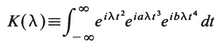
(3.5)
We claim that λt3 and λt4 are small compared to 1 and will use a self consistency argument to demonstrate the point. Supposing they are small, K(λ) can be written

(3.6)
*Dropping regions of t in which ƒ′(t)≠0 can be justified as follows. If ƒ′(t) α≤ t ≤ β, then we can make the change of variables z =ƒ(t). Thus

where

Assuming that ϕ is differentiable, do an integration by parts to yield

Hence F∝β goes to zero like 1/λ; from (3.4) regions having ƒ′=0 give contributions that decrease like 1/√λ and therefore ultimately dominate.
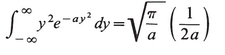
where we have used integration formulas from the appendix to this section. Thus the higher powers of t yield terms that go to zero relative to the first term as λ→∞. Moreover, each factor t2 becomes, after integration, 1/λ. In a sense this means that the effective size of t—or range of t contributing to the integral—is 1/√λ . With this way of counting, λt2 is of order 1, λt3 of order λ-1/2, and so forth.c
To summarize, as λ→∞, the behavior of the integral is determined solely by the point t0 where ƒ′(t0) = 0. Returning to the sum in (3.1), we recall that the correspondence limit is  →0, so we have a parameter λ = 1/ multiplying the function S[x()]. If results about the integral (3.2) mean anything with regard to (3.1), the behavior of the propagator will be dominated by that
  for which δS/δx() = 0. Note that now a functional derivative is in order. But this is precisely the statement that the action is stationary with respect to variation of the path. In this way classical mechanics is recovered and the path
  is found to satisfy the Euler-Lagrange equations.
It is worth mentioning though that although we have found the classical path to be significant in the →0 limit, what is done with it is not the same as is done in classical mechanics. Specifically it is used in a phase factor, so that if there are two classical paths converging on the same region we can still get interference patterns, in contrast to the purely classical prediction.
Of course, to see interference patterns there must be something small compared to . Specifically, suppose there are two classical paths converging on each of the points ξ in some region. Let the associated classical actions for teach ξ be denoted S1(ξ) and S2(ξ). The propagator then has the general form

(3.7)
(actually these terms have real coefficients, which may not be equal). Since the probability distribution is given by |G|2, an interference pattern arises from the effect of the cross term in the product GGc. The cross term is the real part of
ei[S2(ξ)—S1(ξ)]/
Therefore, if the variation in S2 - S1 is large compared to , the pattern will be destroyed by the rapid oscillation of this factor.
Exercise: Suppose a wave function ψ has expectation values for position and momentum x1 and p1, and is sharply concentrated near these values, for example, in a minimum uncertainty wave packet. Let the system evolve under the Hamiltonian H=p2/2m+ V from time t1, to time t2. Show that for →0, at time t2 the wave function will be concentrated at x2, p2 where these are the values of position and momentum the classical system would have reached at t2, starting at x1,p1 at t1.
Solution (very heuristic): Take
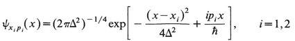
(3.8)
What’s needed is the propagator for a time interval T=t2-t1 and we guess (an educated guess) by analogy with (3.4) that it will take the form

(3.9)
with Sc the value of the action along the path x for which δS=0 and with the appropriate boundary conditions. Moreover, C should be related to the second derivative of S but its exact form is not needed for the purpose of this exercise. What must be shown is that the amplitude

is zero except when x2, p2 is the position in phase space at time t=t1+T of a particle leaving x1,p1 at t=t1. Then from (3.8) and (3.9)
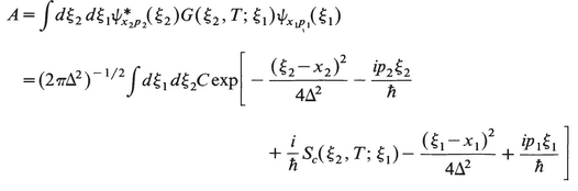
For uncertainties in x and p to be about the same size it is convenient to take  2=O(). For the major contribution to the integral we look to the regions where ∂/∂ξ1, and ∂/∂ξ2 of the argument of the exponent vanish. Keeping ξ1, and ξ2 real, there are the separate requirements that
ξ2=x2 ξ1=x1
and

(3.10)
This says that (P2, x2) and (p1, x1) are related to each other by the canonical transformation generated by the function Sc. But Sc, generates (classically) time evolution, and we have obtained the condition that the particle stick to the classical trajectory. Just how closely it sticks is also implicit in these integrals.
Closely related to the method of stationary phase is Laplace’s method, which deals with integrals of the form

(3.11)
with λ and g real. For g smooth and bounded from below points where g′(x)=0, g″(x)>0 give the greatest contribution. Because of the smallness of the exponential for large λ and g away from its minimum it is easier to prove asymptotic properties for G of (3.11) than for the F of (3.2) as λ→∞. Laplace’s method is dealt with in greater detail in Section 11.
APPENDIX: USEFUL INTEGRALS

(3.12)
(3.13)

(3.14)
(3.15)

(3.16)

(3.17)
(3.18)
For Re a not positive these formulas can be interpreted by analytic continuation, the only complication being a branch point at a= 0.
NOTES
A standard source on asymptotic approximations is
A. Erdelyi, Asymptotic Expansions, Dover, New York, 1956
Additional references are given later in the book when we take up the subject of stationary phase and other asymptotic approximations in a more systematic way. At that stage we also discuss the extent to which the arguments given here can be rigorously applied to path integrals. The problem posed in the exercise of this section has been rigorously solved using methods closely related to the path integral, namely the Trotter product formula. See
G. A. Hagedorn, Semiclassical Quantum Mechanics I: The →0 Limit for Coherent States, Commun. Math. Phys. 71, 77 (1980)