TWENTY

Geometrical Optics

Mathematically speaking, electromagnetism and the nonrelativistic quantum mechanics of a spinless particle differ in two important ways. First, the electromagnetic field is a vector field. Second, it satisfies a partial differential equation of second order in time, in fact hyperbolic, while quantum mechanics is first order in time and parabolic. As far as path integrals are concerned the vector character of the electromagnetic field is indeed a drawback and the would be path integrator of the electromagnetic field is faced by the same challenges discussed later in this book in connection with the path integration of quantum mechanical particles with spin. For this reason, in our treatment of the electromagnetic field we treat it as a scalar quantity—a good deal of useful optics can be understood with this simplified treatment. (Note that we are here discussing a path integral for the electromagnetic wave equation—not the second quantization of the electromagnetic field, which is another matter altogether.)

A way around the fact that the electromagnetic field satisfies a wave equation which is second order in time can be found through a formal trick reminiscent of the way Feynman quantized the Klein-Gordon equation (Section 25).

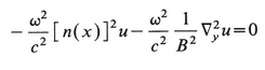
Consider, then, free electromagnetic radiation moving through a medium with a spatially slowly varying index of refraction n(x). Then the “scalar electromagnetic field” u(x, t) satisfies the equation

(20.1)

Consider only waves of a definite frequency ω, so that

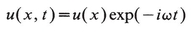
(20.2)

One must be especially careful in defining what parameter will become large in the forthcoming geometrical optics approximation. In fact characteristic distances are large compared to the wavelength of light. Hence when x is measured in units of light wavelengths it will be large, and we are motivated to define

(20.3)

where y is a new variable with characteristic size unity while B→∞ will be the geometrical optics limit. Combining the foregoing equations gives

(20.4)

with 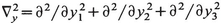. For expositional convenience we assume we are in a situation where n(x)²→E as x→∞, with E some constant (E=1 for vacuum). Define

(20.5)

Equation 20.4 becomes

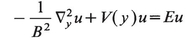
(20.6)

which, one must admit, is beginning to look like Schrödinger’s equation. The next transformation has a very artificial look to it, but it’s what it takes to get the job done, and, if one bears in mind Feynman’s way of dealing with Klein-Gordon particles, is not all that unexpected. Write

(20.7)

The function Ψ, clearly satisfies

(20.8)

so that the parallel to the time dependent Schrödinger equation is manifest. Moreover, the limits →0 and B→∞ are formally identical. On the other hand, to recover a solution of (20.6) from a solution of (20.8) one integrates

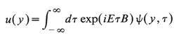
(20.9)

At this stage one can write down a path integral solution for Ψ, but some conceptual clarity is gained by backtracking to (20.6) and considering the Green’s function for that equation, that is, the solution to

(20.10)

in precise analogy to (7.8). As in Section 7, Im E > 0 will provide a convergence factor whenever necessary. (b, a; E) represents a solution to the optics problem in that it gives the illumination at b for a point source at a. It can also be used for the “scattering problem,” that is, to find the scattered wave for a given incoming wave, just as in the quantum mechanical Lippmann Schwinger equation.

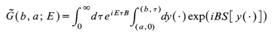
Now the way is clear. The time independent Green’s function G(b, a; E) is obtained from the time dependent one exactly as in Section 7, namely by integration, but with range of integration 0 ≤ τ ≤ ∞ rather than - ∞ to ∞ as in (20.9). The time dependent Green’s function is given by the path integral, and we have finally

(20.11)

with

(20.12)

where the notation dy(·) has been used for “volume in path space” to help us slide the more easily through our hand waving arguments. The notation indicates that only paths satisfying y(0) = a, y(τ) = b are to be summed over. Of course 1/ has everywhere been replaced by B.

For the multiple integral (20.11) the large value of B indicates the use of the stationary phase approximation. The integrals are over τ and y(·), and the argument of the exponent is

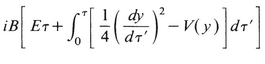
(20.13)

This quantity is to be stationary with respect to variation of both τ and y(·). Variation with respect to y(·) gives the Euler-Lagrange equations and a “classical” path (τ) in the unphysical variable τ, while variation of

(20.14)

which says that the “energy” constant along the path is just E.i

To formulate a variational principle for y(τ) without the unphysical variable τ, we make use of (20.14) to rewrite (20.13) as

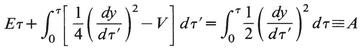
(20.15)

It now follows that among paths satisfying (for all τ’)

(20.16)

which begin at a and end at b, allowing the final time τ to vary also, the classical path (·) is that which makes the quantity

(20.17)

stationary. The freedom to vary τ comes about because with (20.16) given as a constraint, (20.14) becomes the condition that fixes τ.

But the variational principle just formulated is that of Maupertuis. To get rid of the τ in the formulation of the problem we observe that the arc length ds′ along y(s′) is given by

(20.18)

which is of course independent of τ. Moreover, (20.16) can be rewritten as

(20.19)

Substituting,

(20.20)

where s in the integration limit is the length of the path in physical space. We now recall the definition of V, (20.5), so that (E − V)^1/2 is just n(x), which is proportional to 1/υ(x) the local light velocity in the medium.

We can now formulate our conclusion as follows: The path x(s′) (parametrized by arc length s′) which gives the largest contribution to the illumination at a point b from a point source at a is that which makes stationary the integral

(20.21)

among paths x(s′) beginning at a and ending at b, but with total arc lengths not specified.

This is Fermat’s principle! T is just the travel time for the light ray, and our demand is for the path of minimum (stationary, actually) time.

Several comments are in order. First, the stationary path alone does not really give the “largest contribution,” but the paths near it do. I allowed myself some license to make the statement of the conclusion more dramatic. Second, the Gaussian integral around the stationary path can be done, just as for path integrals, and gives the ray density—certainly an important quantity in applications. Third, the entire range of interference and diffraction phenomena is easily handled with this formalism. In case there are two or more stationary solutions there will be interference. When solutions are “close” in function space focusing and caustics exist, exactly as was treated in other sections of this book. Finally it may happen that no solutions exist but that by analytic continuation complex times or complex paths may be found that are stationary. Such “complex paths” suggest a relation to geometric diffraction theory, and were it not for the formal nature of our stationary phase approximation for the path integral the way would be open to a good deal of useful mathematics.

NOTES

The derivation given in this section, or some variant thereof, must surely have been known in the early days of path integrals. So although I doubt that what has been presented here is original, I do not know of any source for it. One paper based on a similar approach is that of

M. Eve, The Use of Path Integrals in Guided Wave Theory, Proc. Roy. Soc. Lond. A 347, 405 (1976)

Geometrical optics of course has its own extensive literature. Ultimately its mathematical justification depends on the stationary phase approximation. I am unable to provide a complete or balanced guide to the literature, but the following papers will at least give the interested reader a handle on further sources:

C. S. Morawetz and D. Ludwig, An Inequality for the Reduced Wave Operator and the Justification of Geometrical Optics, Comm. Pure and Appl. Math. 21, 187 (1968)

D. Ludwig, Uniform Asymptotic Expansions at a Caustic, Comm. Pure and Appl. Math. 19, 215 (1966)

R. A. Handelsman and N. Bleistein, Asymptotic Expansions of Integral Transforms with Oscillatory Kernals: A Generalization of the Method Stationary Phase, SIAM J. Math. Anal. 4, 519 (1973)

“Geometrical diffraction”, a seeming contradiction in terms, is described in

J. B. Keller, Geometrical Theory of Diffraction, J. Opt. Soc. 52, 116 (1962)

Keller has found a way to use ray optics methods in the analysis of diffraction, and it has been suggested that further understanding of his method could come from the sort of path integral approach described in this section.