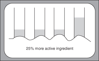
FIGURE 9.1. Misleading baseline data makes true comparisons impossible.
Chapter 9
Interpreting Reports
Smoking is one of the leading causes of statistics.
—Fletcher Knebel
All of who drink of this treatment recover in a short time, except those whom it does not help, who all die. It is obvious, therefore, that it only fails in incurable cases.
—Galen 129–199
THE PREVIOUS CHAPTER WAS AIMED AT PRACTITIONERS WHO must prepare reports. This chapter is aimed at those who must read them, including editors of journals and those who review articles for publication.
Critics may complain we advocate interpreting reports not merely with a grain of salt but with an entire shaker; so be it. Internal as well as published reports are the basis of our thought processes, not just our own publications. Neither society nor we can afford to be led down false pathways.
We are often asked to testify in court or to submit a pretrial declaration in which we comment on published reports. Sad to say, too often the reports our clients hand us lack even the most basic information such as sample sizes, measures of variability, and descriptions of statistical methods, and this despite their having appeared in refereed publications! Most misleading is when we are provided with the results of a statistical analysis but are denied access to the underlying raw data. Monsanto conducted toxicity trials of the company’s broad-spectrum herbicide Roundup. The three animal-feeding studies were conducted in two different laboratories and at two different dates: at Monsanto (Missouri, USA) for NK 603 and MON 810 (June 7, 2000), and at Covance Laboratories Inc. (Virginia, USA) for MON 863 (March 14, 2001) on behalf of Monsanto. Published reports did not include the supporting data or the details of their experimental design.
The raw biochemical data, necessary to allow a statistical reevaluation, were only obtained through court actions (lost by Monsanto) to obtain the MON 863 feeding study material (June 2005), or by courtesy of governments or Greenpeace lawyers (see Vendômois et al., 2009).
Once the raw data are in hand, problems in their interpretation immediately emerged. The reference or control samples had been fed a wide variety of nongenetically modified feeds. These feeds differed in the available amounts of sugars, ions, salts, and pesticide residues. The diets fed to the control and reference groups were not shown to be free of genetically modified feed. Published results were limited to tests of a single variable. Their tests were limited to two samples of ten animals each; thus, the underpowered study had only a 44% chance of detecting a difference as large as one standard deviation.
Begin your appraisal with the authors’ affiliations: Who conducted this study? What is their personal history conducting other studies? What personal interest might they have in the outcome?
Who funded the study? What is the funding agency’s history regarding other studies, and what is their interest in the outcome?
Henschke et al. [2006] reported that screening via computerized tomography increased the chances of early detection of lung cancer. The authors reported, correctly, that their research had been funded by 32 different entities, one of which was the Foundation for Lung Cancer: Early Detection, Prevention, and Treatment. They did not divulge that this foundation was headed by the principal investigator of the 2006 study, that it was housed at her academic institution, and that the only contributor during most of its existence was the Vector Group, the parent company of Liggett, a major tobacco company, that could have an interest in the study results.
Another excellent example is the report of Marshall et al. [2011] on medically supervised injecting facilities and the subsequent rebuttal by Pike et al. [2011]. The authors of the former reference are employed by government health agencies and academic institutions. The authors of the latter, a report that was not peer reviewed, are employees of institutes dedicated to promoting “traditional values,” opposing the legalization of drugs.
Should the study have been performed in the first place? That is, did its potential benefits outweigh the costs to its human or animal subjects?
In a later review of Henske et al. [2006], Leon Gordis raised the following objections:
Several years ago, Dr. Good was asked to analyze the results of a very large-scale clinical study of a new vaccine conducted by the U.S. Department of Defense. He had not been part of the design team, and when he read over the protocol, he was stunned to learn that the design called for inoculating and examining 100,000 servicemen and women, 50,000 with the experimental vaccine, and 50,000 controls with a harmless saline solution.
Why so many? The disease at which the vaccine was aimed was relatively rare. In essence, the study would be comparing two Poisson distributions. Suppose we could expect 0.8% or 400 of the controls to contract the disease, and 0.7% or 350 of those vaccinated to contract it. 100,000 innoculations with their accompanying side effects would yield an expected number of cases of 750.
Could such a study really be justified?
What population(s) was/were sampled from? Were these the same populations to which the report(s) conclusions were applied?
For example, studies of the possibilities of whiplash resulting from low-speed rear-end collisions would only be relevant to specific court cases if the subjects of the studies were of the same age, physical condition, and history of prior injuries as the subjects in the court cases, and if the speeds of impact and the masses and protective ability of the vehicles involved were the same in both the studies and the court cases.
How large was the sample? This most basic piece of information is lacking from the report by Okano et al. [1993]. Was the sample random, stratified, or clustered? What was the survey unit? Was the sample representative? Can you verify this from the information provided in the report?
For example, when several groups are to be compared, baseline information for each group should be provided. A careful reading of Fujita et al. [2000] reveals that the baseline values (age and bone density) of the various groups were quite different, casting doubt on the reported findings.
How was the sample size determined? Was the anticipated power stated explicitly? Without knowledge of the sample size and the anticipated power of the test, we will be unable to determine what interpretation, if any, ought be given a failure to detect a statistically significant effect.
What method of allocation to subgroup was used? What type of blinding was employed, if any? How was blinding verified?
With regard to surveys, what measures were taken to ensure that the responses of different individuals were independent of one another or to detect lies and careless responses? Were nonresponders contacted and interviewed?
Are the authors attempting to compare or combine samples that have been collected subject to different restrictions and by different methods?
Just as the devil often quotes scripture for his (or her) own purposes, politicians and government agencies are fond of using statistics to mislead. One of the most common techniques is to combine data from disparate sources. Four of the six errors reported by Wise [2005] in the presentation of farm statistics arise in this fashion. (The other two come from employing arithmetic means rather than medians in characterizing highly skewed income distributions.) These errors are:
If a study is allegedly double-blind, how was the blinding accomplished? Are all potential confounding factors listed and accounted for?
Is all the necessary information present? Were measures of dispersion (variation) included as well as measures of central tendency? Was the correct and appropriate measure used in each instance: mean (arithmetic or geometric) or median, standard deviation or standard error or bootstrap CI?
Are missing data accounted for? Does the frequency of missing data vary among treatment groups?
Beware of graphs using arbitrary units or with misleading scales. Jean Henrick Schön, whose fraudulent reports wasted many investigators’ time and research monies, used such meaningless graphs with remarkable regularity [Reich, 2009].
Authors must describe which test they used, report the effect size (the appropriate measure of the magnitude of the difference, usually the difference or ratio between groups; a confidence interval would be best), and give a measure of significance, usually a p value, or a confidence interval for the difference.
As Robert Boyle declared in 1661, investigations should be reported in sufficient detail that they can be readily reproduced by others. If the proposed test is new to the literature, a listing of the program code used to implement the procedure should be readily available; either the listing itself or a link to the listing should be included in the report. Throughout the past decade, Salmaso [2002] and his colleagues made repeated claims as to the value of applying permutation methods to factorial designs. Yet not once have these authors published the relevant computer code so that their claims could be verified and acted upon. Berger and Ivanova [2002] claim to have developed a more powerful way to analyze ordered categorical data, yet again, absent their program code, we have no way to verify or implement their procedure.
Can you tell which tests were used? Were they one-sided or two-sided? Was this latter choice appropriate? Consider the examples we listed in Tables 6.1a,b and 6.2. You may even find it necessary to verify the p-values that are provided. Thomas Morgan (in a personal communication) notes that many journal editors now insist that authors use two-tailed tests. This bizarre request stems from the CAST investigation in which investigators ignored the possibility (later found to be an actuality) that the drugs they were investigating were actually harmful. (See Moore, 1995, pp. 203–204; and Moyé, 2000, pp. 145–148 for further details.) Ignoring this possibility had dangerous consequences.
The CAST study is an exception. The majority of comparative studies have as their consequence either that a new drug or process will be adopted or that it will be abandoned, and a one-sided test is justified.
A second reason to be cautious is that the stated p-values may actually be fraudulent. Such would be the case if the choice between a one-tailed and a two-tailed test were made after the data were in hand (UGDP Investigation, 1971) or the authors had computed several statistics (e.g., both the t-test and the Mann–Whitney).
How many tests? In a study by Olsen [2003] of articles in Infection and Immunity, the most common error was a failure to adjust or account for multiple comparisons. Remember, the probability is 64% that at least one test in 20 is likely to be significant at the 5% level by chance alone. Thus, it is always a good idea to check the methods section of an article to see how many variables were measured. See O’Brien [1983], Saville [1990], Tukey [1991], Aickin and Gensler [1996], and Hsu [1996], as well as the minority views of Rothman [1990] and Saville [2003].
Was the test appropriate for the experimental design? For example, was a matched-pairs t-test used when the subjects were not matched?
Note to journal editors: The raw data that formed the basis for a publication should eventually be available on a website for those readers who may want to run their own analyses.
Was an exact method used for their analysis or a chi-square approximation? Were log-linear models used when the hypothesis of independence among diverse dimensions in the table did not apply?
Was factor analysis applied to datasets with too few cases in relation to the number of variables analyzed? Was oblique rotation used to get a number of factors bigger or smaller than the number of factors obtained in the initial extraction by principal components, as a way to show the validity of a questionnaire? An example provided by Godino, Batanero, and Gutiérrez-Jaimez [2001] is obtaining only one factor by principal components and using the oblique rotation to justify that there were two differentiated factors, even when the two factors were correlated and the variance explained by the second factor was very small.
One should always be suspicious of a multivariate analysis, both of the methodology and of the response variables employed. While Student’s-t is very robust, even small deviations from normality make the p-values obtained from Hotelling’s T2 suspect. The inclusion of many irrelevant response variables may result in values that are not statistically significant.
Always look for confidence intervals about the line. If they are not there, distrust the results unless you can get hold of the raw data and run the regressions and a bootstrap validation yourself (see Chapters 13 and 14).
Beware of missing baselines, as in Figure 9.1. Be wary of extra dimensions that inflate relative proportions (see Chapter 10). Distrust curves that extend beyond the plotted data. Check to see that charts include all datapoints, not just some of them.
FIGURE 9.1. Misleading baseline data makes true comparisons impossible.

The data for Figure 9.2, supplied by the California Department of Education, are accurate. The title added by an Orange County newspaper is not. Although enrollment in the Orange County public schools may have been steadily increasing in the last quarter of the 20th Century, clearly it has begun to level off and even to decline in the 21st.
FIGURE 9.2. Enrollment in Orange County Public Schools from 1977 to 2007.
Source: California Department of Education. The misleading title was added by an Orange County newspaper. Data are downloadable from http://www.cde.ca.gov/ds/sd/sd.
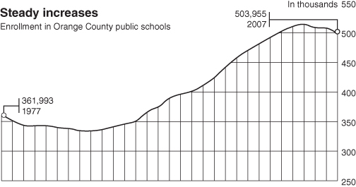
Finally, as noted in the next chapter, starting the Y-axis at 250,000 rather than 0 leaves the misleading impression that the increase is much larger than it actually is.
Our greatest fault (apart from those to which our wives have been kind enough to draw our attention) is to save time by relying on the abstract and/or the summary of a paper for our information, rather than wade through the entire article. After all, some reviewer has already gone through it with a fine-tooth comb. Or have they? Most reviewers, though experts in their own disciplines, are seldom as knowledgeable in statistics. It is up to us to do the job, to raise the questions that ought to have been asked before the article was published.
Is an attempt made to extend results beyond the populations that were studied? Are potential biases described?
Were any of the tests and subgroup analyses performed after the data were examined, thereby rendering the associated p-values meaningless? And, again, one must ask, were all potential confounding factors accounted for either by blocking or by treatment as covariates? (See, for example, the discussion of Simpson’s paradox in Chapter 11.)
Be wary of extrapolations, particularly in multifactor analyses. As the small print reads on a stock prospectus, past performance is no guarantee of future success.
Are nonsignificant results taken as proof of lack of effect? Are practical and statistical significance distinguished?
Finally, few journals publish negative findings, so avoid concluding that “most studies show.”
Consider the statement “Sixty percent of the children in New York City read below grade level.” Some would say we can not tell whether this percentage is of practical significance without some means of comparison. How does New York City compare with other cities its size? What about racial makeup? What about other environmental factors compared with other similar cities?
In the United States in 1985, there were 2.1 million deaths from all causes, compared to 1.7 million in 1960. Does this mean it was safer to live in the United States in the 1960s than in the 1980s? We do not know the answer because we do not know the relative sizes of the population of the United States in 1960 and 1985.
If a product had a 10% market share in 1990 and 15% today, is this a 50% increase or a 5% increase? Not incidentally, note that market share may increase even when total sales decline.
How are we to compare rates? If a population consists of 12% African-Americans, and a series of jury panels contain only 4%, the absolute disparity is 8%, but the comparative disparity is 66%.
In Davis v. City of Dallas4, the court observed that a “7% difference between 97% and 90% ought not to be treated the same as a 7% difference between, e.g. 14% and 7%, since the latter figure indicates a much greater degree of disparity.” Not so, for pass rates of 97% and 90% immediately imply failure rates of 3% and 10%.
The consensus among statisticians is that one ought use the odds ratio for such comparisons, defined as the percentage of successes divided by the percentage of failures. In the present example, one would compare 97%/3% = 32.3 versus 90%/10% = 9. Katz [2006] dissents.
Many of our reports come to us directly from computer printouts. Even when we are the ones who have collected the data, these reports are often a mystery. One such report, generated by SAS PROC TTEST is reproduced and annotated below. We hope our annotations will inspire you to do the same with the reports your software provides you. (Hint: Read the manual.)
First, a confession: We have lopped off many of the decimal places that were present in the original report. They were redundant as the original observations only had two decimal places. In fact, the fourth decimal place is still redundant.
Second, we turn to the foot of the report, where we learn that a highly significant difference was detected between the dispersions (variances) of the two treatment groups. We will need to conduct a further investigation to uncover why this is true.
Confining ourselves to the report in hand, unequal variances mean that we need to use the Satterthwaite’s degrees of freedom adjustment for the t-test for which Pr > |t| = 0.96, that is, the values of RIG for the New and Standard treatment groups are not significantly different from a statistical point of view.
Lastly, the seventh line of the report tells us that the different in the means of the two groups is somewhere in the interval (−0.05, +0.05). (The report does not specify what the confidence level of this confidence interval is and we need to refer to the SAS manual to determine that it is 95%.)
 The TTEST Procedure
 Statistics
 Lower CL Upper CL Lower CL Upper CL
Var'le treat N Mean Mean Mean Std Dev Std Dev Std Dev Std Err
RIG New 121 0.5527 0.5993 0.6459 0.2299 0.2589 0.2964 0.0235
RIG Stand 127 0.5721 0.598 0.6238 0.1312 0.1474 0.1681 0.0131
RIG Diff (1–2)–0.051 0.0013 0.0537 0.1924 0.2093 0.2296 0.0266
 T-Tests
Variable Method Variances DF t Value Pr > |t|
RIG Pooled Equal 246 0.05 0.9608
RIG Satterthwaite Unequal 188 0.05 0.9613
Equality of Variances
Variable Method Num DF Den DF F Value Pr > F
RIG Folded F 120 126 3.09 <.0001
I just wanted to make something more beautiful than it is.
—Translation of a remark by G. Stapel
If the numerous surveys cited by Judson [2004] are accurate, 10–15% of scholarly publications include either made-up or “modified” data. Sometimes, the fraud leaps out at the reader (though not, apparently, at the reviewers for the journals in which the articles appeared). Between 1943 and 1966, Sir Cyril Burt (he was knighted for his work in psychology) published a series of papers on the differences between pairs of twins who had been reared together and pairs of twins who had been reared apart. The numbers of pairs of twins for whom data were collected increased over time, though the raw data were never reported (nor, in those pre-Internet days, were data made available online to other investigators). The following table summarizes Burt’s and his coauthor’s reported findings:
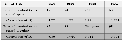
What a coincidence! Correlations that remain constant to three decimal places.
A less obvious anomaly of Burt’s statistical analyses was that his recorded p-values for the chi-square statistic were all highly insignificant, that is, they exceeded the 99th percentile of the distribution.
Between December 2011 and January 2012, the U.S. Department of Labor reported a statistically adjusted gain of 243,000 jobs in January 2012, whereas the raw actual jobs numbers showed an actual loss of 2.7 million jobs.
Jack Rasmus suggests that the Labor Department may be using methods and assumptions based on conditions that pre-dated the current recession’s unique, qualitatively different, and more–severe conditions.
Jan Henrick Schon’s fraud was exposed, in part, because Lydia Sohn and Paul McEuen noticed that the graphs in several of Schon’s articles were so similar that even the little wiggles due to random fluctuations were the same!
The respected Nathan Mantel wrote in 1979 to editors of Biometrics to question certain simulation results on the grounds that the values seemed to bounce around rather than fall on a smooth curve. Now that we are more familiar with the use of simulations in statistics, a more obvious question would be why so many reported results were so smooth, when surely one or two outliers are always to be expected. The only way one can verify simulation results or extend them to distributions of particular interest is if one has access to the code that generated results; journal editors should require the code’s publication.
While one’s intuition might suggest that each of the numbers 1 through 9 is equally likely to be one of the leading digits in a table entry, if the data are distributed across several orders of magnitude, the probability that a leading digit is k is given by the formula P[k] = log[1 + 1/k].
The formula, known as Benford’s Law had been known in one form or another for more than a century. Varian [1972] was among the first to suggest that it might be applied to the analysis of scientific data.
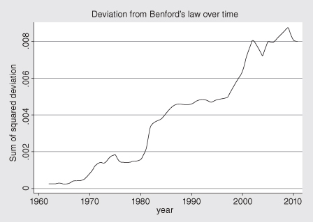
Using quarterly accounting data for all firms in Compustat, Jialan Wang found that accounting statements are getting less and less representative of what is really going on inside of companies (see Figure 9.3). The major reform that was passed after Enron and other major accounting scandals barely made a dent.
FIGURE 9.3. Deviations from Benford’s Law for accounting data for 20,000 firms as a function of time.
Source: Jialan Wang as reported at http://economistsview.typepad.com/economistsview/2011/10/benfords-law-and-the-decreasing-reliability-of-accounting-data.html.
Reports of scientific endeavors should be comprehensive enough to permit the reader to replicate the procedures described therein and to confirm or challenge the reported results.
Godino, Batanero, and Gutiérrez-Jaimez [2001] report on errors found in the use of statistics in a sample of mathematics education doctoral theses in Spain. Fanelli [2009] and Martinson, Anderson, and Devries [2005] report on the prevalence of fraud. Durtschi et al. [2004] report on the use of Benford’s Law to detect fraud.
Notes
1 Eagle Iron Works, 424 F. Supp, 240 (S.D. Ia. 1946).
2 185 F.2d 258 (4th Cir. 1950).
3 Amstar Corp. v. Domino’s Pizza, Inc., 205 U.S.P.Q 128 (N.D. Ga. 1979), rev’d, 615 F. 2d 252 (5th Cir. 1980).
4 487 F.Supp 389 (N.D. Tex 1980).