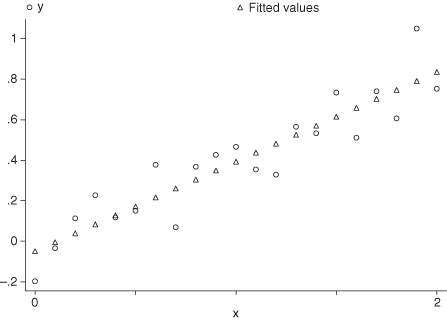
FIGURE 11.1. A straight line appears to fit the data.
Chapter 11
Univariate Regression
Are the data adequate? Does your data set cover the entire range of interest? Will your model depend on one or two isolated datapoints?
THE SIMPLEST EXAMPLE OF A MODEL, THE RELATIONSHIP between exactly two variables, illustrates at least five of the many complications that can interfere with the task of model building:
We consider each of these error sources in turn along with a series of preventive measures. Our discussion is divided into problems connected with model selection and difficulties that arise during the estimation of model coefficients.
Almost every relationship has both a linear and a nonlinear component with the nonlinearities becoming more evident as we approach the extremes of the independent (causal) variable’s range. One can think of many examples from physics, such as Boyles Law, which fails at high pressure, and particle symmetries that are broken as the temperature falls.
Almost every measuring device—electrical, electronic, mechanical, or biological—is reliable only in the central portion of its scale. In medicine, a radioimmune assay fails to deliver reliable readings at very low dilutions; this has practical implications as an increasing proportion of patients will fail to respond as the dosage drops.
We need to recognize that although a regression equation may be used for interpolation within the range of measured values, we are on shaky ground if we try to extrapolate, to make predictions for conditions not previously investigated. The solution is to know the range of application and to recognize, even if we do not exactly know the range, that our equations will be applicable to some but not all possibilities.
Think why rather than what.
The exact nature of the formula connecting two variables cannot be determined by statistical methods alone. If a linear relationship exists between two variables X and Y, then a linear relationship also exists between Y and any monotonic (nondecreasing or nonincreasing) function of X. Assume X can only take positive values. If we can fit Model I—Y = α + βX + ε—to the data, we also can fit Model II—Y = α′ + β′log[X] + ε—and Model III—Y = α″ + β″X + γX2 + ε. It can be very difficult to determine which model if any is the “correct” one in either a predictive or mechanistic sense.
A graph of Model I is a straight line (see Figure 11.1). Because Y includes a stochastic or random component ε, the pairs of observations (x1, y1), (x2, y2), … will not fall exactly on this line but above and below it. The function log[X] does not increase as rapidly as X does. When we fit Model II to these same pairs of observations, its graph rises above that of Model I for small values of X and falls below that of Model I for large values. Depending on the set of observations, Model II may give just as good a fit to the data as Model I.
FIGURE 11.1. A straight line appears to fit the data.

How Model III behaves will depend upon whether β″ and α″ are both positive or whether one is positive and the other negative. If β″ and α″ are both positive, then the graph of Model III will lie below the graph of Model I for small positive values of X and above it for large values. If β″ is positive and α″ is negative, then Model III will behave more like Model II. Thus Model III is more flexible than either Models I or II and can usually be made to give a better fit to the data, that is, to minimize some function of the differences between what is observed, yi, and what is predicted by the model, Y[xi].
The coefficients α, β, and γ for all three models can be estimated by a technique known (to statisticians) as linear regression. Our knowledge of this technique should not blind us to the possibility that the true underlying model may require nonlinear estimation as in

This latter model may have the advantage over the first three in that it fits the data over a wider range of values.
Which model should we choose? At least two contradictory rules apply:
Again, the best rule of all is not to let statistics do your thinking for you, but to inquire into the mechanisms that give rise to the data and that might account for the relationship between the variables X and Y. An example taken from physics is the relationship between volume V and temperature T of a gas. All of the preceding four models could be used to fit the relationship. But only one, the model V = a + KT, is consistent with kinetic molecular theory.
An example in which the simpler, more straightforward model is not correct arises when we try to fit a straight line to what is actually a higher-order polynomial. For example, suppose we try to fit a straight line to the relationship Y = (X − 1)2 over the range X = (0, +2). We would get a line with slope 0, similar to that depicted in Figure 11.2. With a correlation of 0, we might even conclude in error that X and Y were not related. Figure 11.2 suggests a way we can avoid falling into a similar trap.
FIGURE 11.2. Fitting an inappropriate model.
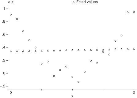
Always plot the data before deciding on a model.
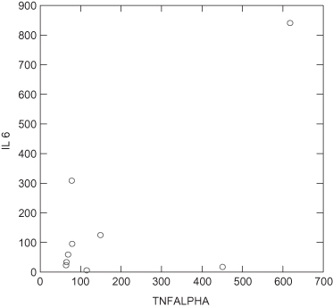
The data in Figure 11.3 are taken from Mena et al. [1995]. These authors reported in their abstract that “The correlation … between IL-6 and TNF-alpha was .77, … statistically significant at a p-value less than .01.” Would you have reached the same conclusion?
FIGURE 11.3. Relation between two inflammatory reaction mediators in response to silicone exposure.
Data taken from Mena et al [1995].
With more complicated models, particularly those like Model IV that are nonlinear, it is advisable to calculate several values that fall outside the observed range. If the results appear to defy common sense (or the laws of physics, market forces, etc.) the nonlinear approach should be abandoned and a simpler model utilized.
Often, it can be difficult to distinguish which variable is the cause and which the effect. But if the values of one of the variables are fixed in advance, then this variable should always be treated as the so-called independent variable or cause, the X in the equation Y = a + bX + ε. Here is why.
When we write Y = a + bx + ε, we actually mean Y = E(Y|x) + ε, where E(Y|X) = a + bx is the expected value of an indefinite number of independent observations of Y when X = x. If X is fixed, the inverse equation x = (E(x|Y) − a)/b + ε′ = makes little sense.
Though a model may provide a good fit to a set of data, one ought refrain from inferring any causal connection. The reason is that a single model is capable of fitting many disparate data sets. Consider that one line, Y = 3 + 0.5X, fits the four sets of paired observations depicted in Figures 11.4a, b, c, and d with R2 = 0.67 in each case.
FIGURE 11.4. The best fitting (regression) line for each of these four datasets is y = 3 + .5x where each regression is characterized by R2 = 0.67. The upper-left plot is a reasonable dataset for which the linear model is applied. The upper-right plot illustrates a possible quadratic relationship not accounted for by our linear model; the lower left demonstrates the effect of a possibly miscoded outcome value yielding a slope that is somewhat higher than it otherwise would be, while the lower right demonstrates an outlier that markedly alters the slope of the line.
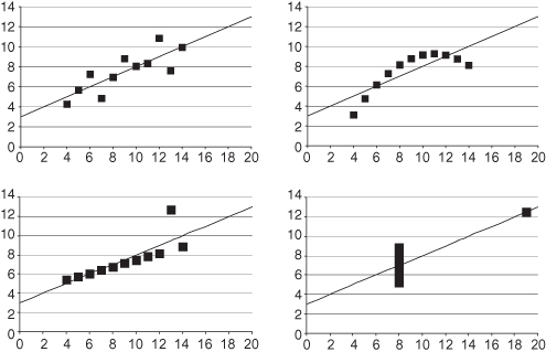
The data for these four figures are as follows:
If the effects of additional variables other than X on Y are suspected, these additional effects should be accounted for either by stratifying or by performing a multivariate regression.
Correlations can be deceptive. Variable X can have a statistically significant correlation with variable Y solely because X and Y are both dependent on a third variable Z. A fall in the price of corn is inversely proportional to the number of hay-fever cases only because the weather that produces a bumper crop of corn generally yields a bumper crop of ragweed as well.
Even if the causal force X under consideration has no influence on the dependent variable Y, the effects of unmeasured selective processes can produce an apparent test effect. Children were once taught that storks brought babies. This juxtaposition of bird and baby makes sense (at least to a child) for where there are houses there are both families and chimneys where storks can nest. The bad air or miasma model (“common sense” two centuries ago) works rather well at explaining respiratory illnesses and not at all at explaining intestinal ones. An understanding of the role that bacteria and viruses play unites the two types of illness and enriches our understanding of both.
We often try to turn such pseudocorrelations to advantage in our research, using readily measured proxy variables in place of their less easily measured “causes.” Examples are our use of population change in place of economic growth, M2 for the desire to invest, arm cuff blood pressure measurement in place of the width of the arterial lumen, and tumor size for mortality. At best, such surrogate responses are inadequate (as in attempting to predict changes in stock prices); in other instances they may actually point in the wrong direction.
At one time, the level of CD-4 lymphocytes in the blood appeared to be associated with the severity of AIDS; the result was that a number of clinical trials used changes in this level as an indicator of disease status. Reviewing the results of 16 sets of such trials, Fleming [1995] found that the concentration of CD-4 rose to favorable levels in 13 instances even though clinical outcomes were only favorable in eight.
Gender discrimination lawsuits based on the discrepancy in pay between men and women could be defeated once it was realized that pay was related to years in service and that women who had only recently arrived on the job market in great numbers simply didn’t have as many years on the job as men.
These same discrimination lawsuits could be won once the gender comparison was made on a years-in-service basis, that is when the salaries of new female employees were compared with those of newly employed men, the salaries of women with three years of service with those of men with the same time in grade, and so forth. Within each stratum, men always had the higher salaries.
If the effects of additional variables other than X on Y are suspected, they should be accounted for either by stratifying or by performing a multivariate regression as described in the next chapter.
The two approaches are not equivalent unless all terms are included in the multivariate model. Suppose we want to account for the possible effects of gender. Let I[] be an indicator function that takes the value 1 if its argument is true and 0 otherwise. Then, to duplicate the effects of stratification, we would have to write the multivariate model in the following form:

In a study by Kanarek et al. [1980] whose primary focus is the relation between asbestos in drinking water and cancer, results are stratified by sex, race, and census tract. Regression is used to adjust for income, education, marital status, and occupational exposure.
Lieberson [1985] warns that if the strata differ in the levels of some third unmeasured factor that influences the outcome variable, the results may be bogus.
A third omitted variable may also result in two variables appearing to be independent when the opposite is true. Consider the following table, an example of what is termed Simpson’s paradox:
| Treatment Group | ||
| Control | Treated | |
| Alive | 6 | 20 |
| Dead | 6 | 20 |
We do not need a computer program to tell us the treatment has no effect on the death rate. Or does it? Consider the following two tables that result when we examine the males and females separately:
| Males | ||
| Control | Treated | |
| Alive | 4 | 8 |
| Dead | 3 | 5 |
| Females | ||
| Control | Treated | |
| Alive | 2 | 12 |
| Dead | 3 | 15 |
In the first of these tables, treatment reduces the male death rate from 3 out of 7, or 0.43, to 5 out of 13, or 0.38. In the second table the redaction is from 3 out of 5, or 0.6, to 15 out of 27, or 0.55. Both sexes show a reduction, yet the combined population does not. Resolution of this paradox is accomplished by avoiding a knee-jerk response to statistical significance when association is involved. One needs to think deeply about underlying cause-and-effect relationships before analyzing data. Thinking about cause and effect in the preceding example might have led us to thinking about possible sexual differences, and to stratifying the data by sex before analyzing it.
Write down and confirm your assumptions before you begin.
In this section, we consider problems and solutions associated with three related challenges:
The techniques we employ will depend upon the following:
The estimates we obtain will depend upon our choice of fitting function. Our choice should not be dictated by the software but by the nature of the losses associated with applying the model. Our software may specify a least-squares fit—most commercially available statistical packages do—but our real concern may be with minimizing the sum of the absolute values of the prediction errors or the maximum loss to which one will be exposed. A solution is provided in the next chapter.
In the univariate linear regression model, we assume that

where E denotes the mathematical expectation of Y given x and could be any deterministic function of x in which the parameters appear in linear form. ε, the error term, stands for all the other unaccounted-for factors that make up the observed value y.
How accurate our estimates are and how consistent they will be from sample to sample will depend upon the nature of the error terms. If none of the many factors that contribute to the value of ε make more than a small contribution to the total, then ε will have a Gaussian distribution. If the {εi} are independent and normally distributed (Gaussian), then the ordinary least-squares estimates of the coefficients produced by most statistical software will be unbiased and have minimum variance.
These desirable properties, indeed the ability to obtain coefficient values that are of use in practical applications, will not be present if the wrong model has been adopted. They will not be present if successive observations are dependent. The values of the coefficients produced by the software will not be of use if the associated losses depend on some function of the observations other than the sum of the squares of the differences between what is observed and what is predicted. In many practical problems, one is more concerned with minimizing the sum of the absolute values of the differences or with minimizing the maximum prediction error. Finally, if the error terms come from a distribution that is far from Gaussian, a distribution that is truncated, flattened or asymmetric, the p-values and precision estimates produced by the software may be far from correct.
Alternatively, we may use permutation methods to test for the significance of the resulting coefficients. Providing that the {εi} are independent and identically distributed (Gaussian or not), the resulting p-values will be exact. They will be exact regardless of which goodness-of-fit criterion is employed.
Suppose that our hypothesis is that yi = a + bxi + εi for all i and b = b0. First, we substitute  in place of the original observations yi. Our translated hypothesis is
  for all i and b′ = 0 or, equivalently, ρ = 0, where ρ is the correlation between the variables Y′ and X. Our test for correlation is based on the permutation distribution of the sum of the cross-products
  [Pitman, 1938]. Alternative tests based on permutations include those of Cade and Richards [1996] and MRPP LAD regression [Mielke and Berry, 1997].
For large samples, these tests are every bit as sensitive as the least-squares test described in the previous paragraph even when all the conditions for applying that test are satisfied [Mielke and Berry, 2001; Section 5.4].
If the errors are dependent, normally distributed, and the covariances are the same for every pair of errors, then we may also apply any of the permutation methods described above. If the errors are dependent and normally distributed, but we are reluctant to make such a strong assumption about the covariances, then our analysis may call for dynamic regression models [Pankratz, 1991].1
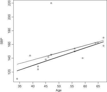
The presence of bad data can completely distort regression calculations. When least-squares methods are employed, a single outlier can influence the entire line to pass closely to the outlier.
Consider the effect on the regression line in Figure 11.5 if we were to eliminate the systolic blood pressure reading of 220 for a 47-year old. The slope increases and the intercept decreases.
FIGURE 11.5. Effect on the Model of Eliminating an Outlying Observation.
Although a number of methods exist for detecting the most influential observations (see, for example, Mosteller and Tukey, 1977), influential does not automatically mean that the data point is in error. Measures of influence encourage review of data for exclusion. Statistics do not exclude data; analysts do. And they only exclude data when presented with firm evidence that the data are in error.
The problem of bad data is particularly acute in two instances:
The Washington State Department of Social and Health Services extrapolates its audit results on the basis of a regression of over- and undercharges against the dollar amount of the claim. As the frequency of errors depends on the amount of paperwork involved and not on the dollar amount of the claim, no causal relationship exists between overcharges and the amount of the claim. The slope of the regression line can vary widely from sample to sample; the removal or addition of a very few samples to the original audit can dramatically affect the amount claimed by the State in overcharges.
Recommended is the delete-one approach in which the regression coefficients are recomputed repeatedly, deleting a single pair of observations from the original dataset each time. These calculations provide confidence intervals for the estimates along with an estimate of the sensitivity of the regression to outliers. When the number of data pairs exceeds a hundred, a bootstrap might be used instead.
To get an estimate of the precision of the estimates and the sensitivity of the regression equation to bad data, recompute the coefficients, leaving out a different data pair each time.
More often than we would like to admit, the variables and data that go into our models are chosen for us. We cannot directly measure the variables we are interested in so we make do with surrogates. But such surrogates may or may not be directly related to the variables of interest. Lack of funds and or/the necessary instrumentation limit the range over which observations can be made. Our census overlooks the homeless, the uncooperative, and the less luminous. (See, for example, City of New York v. Dept of Commerce 2; Disney, 1976; and Bothun, 1998, Chapter 6.)
The presence of such bias does not mean we should abandon our attempts at modeling, but that we should be aware of and report our limitations.
An underlying assumption of regression methods is that relationships among variables remain constant during the data collection period. If not, if the variables we are measuring undergo seasonal or other detectable changes in their means or variances, then we need to account for them.
Most methods of time-series analysis require stationarity. Examples, which also conform to OLS linear regression, include the autoregressive model  and the periodic Serfling method,

where dow stands for day of the week and doy for day of the year.
Stationarity for a time-series analysis can be achieved in two ways:
To assess the predictive value of a model, the observations in the test set must occur after the observations in the training set. A weakness of the Box–Jenkins approach is that multiple models may provide equally good fits to the training set and equally good predictions for the test set. This may suggest that other, unexamined predictors are actually responsible for the changes over time of the variable of interest.
For example, studies suggest that the weather is the best predictor for the volume of warranty repairs on automobiles. Alas, it is no easier to predict the weather than the volume of warranties.
The sensitivity, specificity, and timeliness of detection of a time-series model can be improved upon by adopting one of the methodologies described in Chapter 14; see, for example, Wieland et al. [2007].
An association can be of statistical significance without being of the least practical value. In the study by Kanarek et al. [1980] referenced above, a 100-fold increase in asbestos fiber concentration is associated with perhaps a 5% increase in lung cancer rates. Do we care? Perhaps, for no life can be considered unimportant. But courts traditionally have looked for at least a two-fold increase in incidence before awarding damages. (See, for example, the citations in Chapter 6 of Good, 2001.) And in this particular study, there is reason to believe there might be other hidden cofactors that are at least as important as the presence of asbestos fiber.
As noted above, we have a choice of fitting methods: We can minimize the sum of the squares of the deviations between the observed and model values, or we can minimize the sum of the absolute values of these deviations, or we can minimize some entirely different function. Suppose that we have followed the advice given above and have chosen our goodness-of-fit criterion to be identical with our loss function.
For example, suppose the losses are proportional to the square of the prediction errors, and we have chosen our model’s parameters so as to minimize the sum of squares of the differences yi – M[xi] for the historical data. Unfortunately, minimizing this sum of squares is no guarantee that when we continue to make observations, we will continue to minimize the sum of squares between what we observe and what our model predicts. If you are a businessperson whose objective is to predict market response, this distinction can be critical.
There are at least three reasons for the possible disparity:
And lest we forget: association does not “prove” causation, it can only contribute to the evidence.
The use of an indicator (yes/no) or a nonmetric ordinal variable (improved, much improved, or no change) as the sole independent (X) variable is inappropriate. The two-sample and k-sample procedures described in Chapter 5 should be employed.
It is often the case that the magnitude of the residual error is proportional to the size of the observations, that is, y = E(Y|x)ε. A preliminary log transformation will restore the problem to linear form log(y) = log E(Y|x) + ε′. Unfortunately, even if ε is normal, ε′ is not, and the resulting confidence intervals need be adjusted [Zhou and Gao, 1997].
I have attended far too many biology conferences at which speakers have used a significant linear regression of one variable on another as “proof” of a “linear” relationship or first-order behavior.
Linear or first-order growth occurs when we pour water into a bathtub. At least initially, V = ft, where V is the volume of water in the tub, f is the flow rate, and t is the amount of time that has elapsed since we first turned on the tap.
Second-order growth is characteristic of epidemics, at least initially. As each new case increases the probability of infection, N = at + bt2, where N is the number of infected individuals and t represents time, as before.
Third-order growth is characteristic of political movements and enzyme-coupled reactions, when recruitment of new individuals is active, not merely passive. As with second-order and first-order reactions, should we attempt to fit the equation N = at, the result will be a value of the coefficient a that is significantly different from zero.
The unfortunate fact, which should not be forgotten, is that if EY = a f[X], where f is a monotonically, increasing function of X, then any attempt to fit the equation Y = bg[X], where g is also a monotonically increasing function of X, will result in a value of b that is significantly different from zero. The “trick,” as noted in our first lesson, is in selecting an appropriate (cause-and-effect-based) functional form g to begin with. Regression methods and expensive software will not find the correct form for you.
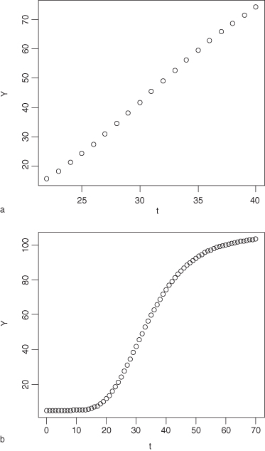
Few processes are purely linear. Almost all have an S-shape, though the lengths of the left and right horizontals of the S may differ. Sometimes, the S-shape results from the measuring instruments, which typically fail for very large or very small values. But equally often, it is because there is a lower threshold that needs be overcome and an upper limit that results from saturation.
For example, in Figure 11.6a, the linear relationship between the dependent variable Y and the time t appears obvious. But as seen in Figure 11.6b, the actual relationship between Y and t is that of logistic growth.
FIGURE 11.6. a. The linear relationship between the dependent variable Y and the time t appears obvious. b. But the actual relationship between Y and t is that of logistic growth.
We have already distinguished processes where the growth is additive with time, y = a + bt, from those where it is multiplicative, y = aebt, and we work instead with the relationship log[y] = a + bt. But the growth of welfare in the 1960s was found to occur in four phases:
In this example, the variable to be predicted is not a measurement but a count, and logistic regression, considered in Chapter 14, would be more appropriate. In this example, we had a plausible explanation.
Until recently, what distinguished statistics from the other branches of mathematics was that at least one aspect of each analysis was firmly grounded in reality. Samples were drawn from real populations and, in theory, one could assess and validate findings by examining larger and larger samples taken from that same population.
In this reality-based context, modeling has one or possibly both of the following objectives:
Failure to achieve these objectives has measurable losses. While these losses cannot be eliminated because of the variation inherent in the underlying processes, hopefully, by use of the appropriate statistical procedure, they can be minimized.
By contrast, the goals of curve fitting (nonparametric, spline fitting, or local regression)3 are aesthetic in nature; the resultant graphs, though pleasing to the eye, may bear little relation to the processes under investigation. To quote Green and Silverman [1994; p. 50], “there are two aims in curve estimation, which to some extent conflict with one another, to maximize goodness-of-fit and to minimize roughness.”
The first of these aims is appropriate if by goodness-of-fit is meant minimizing the loss function.4 In our example of modeling the welfare case load, we could justify each additional parameter on a casual basis. Absent such a basis, merely minimizing roughness creates a strong risk of overfitting.
Validation is essential, yet most of the methods discussed in Chapter 15 do not apply. Validation via a completely independent dataset cannot provide confirmation, as the new data would entail the production of a completely different, unrelated curve. The only effective method of validation is to divide the data set in half at random, fit a curve to one of the halves, and then assess its fit against the entire data set.
Regression methods work well with physical models. The relevant variables are known and so are the functional forms of the equations connecting them. Measurement can be done to high precision, and much is known about the nature of the errors—in the measurements and in the equations. Furthermore, there is ample opportunity for comparing predictions to reality.
Regression methods can be less successful for biological and social science applications. Before undertaking a univariate regression, you should have a fairly clear idea of the mechanistic nature of the relationship (and thus the form the regression function will take). Look for deviations from the model, particularly at the extremes of the variable range. A plot of the residuals can be helpful in this regard; see, for example, Davison and Snell [1991] and Hardin and Hilbe [2002; pp. 143–159].
A preliminary multivariate analysis (the topic of the next two chapters) will give you a fairly clear notion of which variables are likely to be confounded so that you can correct for them by stratification. Stratification will also allow you to take advantage of permutation methods that are to be preferred in instances where “errors” or model residuals are unlikely to follow a normal distribution.
It is also essential that you have firmly in mind the objectives of your analysis, and the losses associated with potential decisions, so that you can adopt the appropriate method of goodness of fit. The results of a regression analysis should be treated with care; as Freedman [1999] notes,
Even if significance can be determined and the null hypothesis rejected or accepted, there is a much deeper problem. To make causal inferences, it must in essence be assumed that equations are invariant under proposed interventions. … [I]f the coefficients and error terms change when the variables on the right-hand side of the equation are manipulated rather than being passively observed, then the equation has only a limited utility for predicting the results of interventions.
Statistically significant findings should serve as a motivation for further corroborative and collateral research rather than as a basis for conclusions.
David Freedman’s [1999] article on association and causation is must reading. Lieberson [1985] has many examples of spurious association. Friedman, Furberg, and DeMets [1996] cite a number of examples of clinical trials using misleading surrogate variables.
Mosteller and Tukey [1977] expand on many of the points raised here concerning the limitations of linear regression. Distribution-free methods for comparing regression lines among strata are described by Good [2001; pp. 168–169].
For a real-world example of Simpson’s paradox, see http://www.stats.govt.nz/searchresults.aspx?q=Simpson’s paradox.
Notes
1 In the SAS manual, these are called ARIMAX techniques and are incorporated in Proc ARIMA.
2 822 F. Supp. 906 (E.D.N.Y., 1993).
3 See, for example Green and Silverman [1994] and Loader [1999].
4 Most published methods also require that the loss function be least-squares and the residuals be normally distributed.