Chapter 12
Alternate Methods of Regression
Imagine how statisticians might feel about the powerful statistics programs that are now in our hands. It is so easy to key-in a set of data and calculate a wide variety of statistics—regardless what those statistics are or what they mean. There also is a need to check that things are done correctly in the statistical analyses we perform in our laboratories.
—James O. Westgard [1998]
IN THE PREVIOUS CHAPTER, WE FOCUSED EXCLUSIVELY ON ordinary least-squares linear regression (OLS) both because it is the most common modeling technique and because the limitations and caveats we outlined there apply to virtually all modeling techniques. But OLS is not the only modeling technique. To diminish the effect of outliers, and treat prediction errors as proportional to their absolute magnitude rather than their squares, one should use least absolute deviation (LAD) regression. This would be the case if the conditional distribution of the dependent variable were characterized by a distribution with heavy tails (compared to the normal distribution, increased probability of values far from the mean).
One should also employ LAD regression when the conditional distribution of the dependent variable given the predictors is not symmetric and we wish to estimate its median rather than its mean value.
If it is not clear which variable should be viewed as the predictor and which the dependent variable, as is the case when evaluating two methods of measurement, then one should employ Deming or error in variable (EIV) regression.
If one’s primary interest is not in the expected value of the dependent variable but in its extremes (the number of bacteria that will survive treatment or the number of individuals who will fall below the poverty line), then one ought consider the use of quantile regression.
If distinct strata exist, one should consider developing separate regression models for each stratum, a technique known as ecological regression, discussed in the next-to-last section of the present chapter.
If one’s interest is in classification or if the majority of one’s predictors are dichotomous, then one should consider the use of classification and regression trees (CART) discussed in the next chapter.
If the outcomes are limited to success or failure, one ought employ logistic regression. If the outcomes are counts rather than continuous measurements, one should employ a generalized linear model (GLM). See Chapter 14.
Linear regression is a much misunderstood and mistaught concept. If a linear model provides a good fit to data, this does not imply that a plot of the dependent variable with respect to the predictor would be a straight line, only that a plot of the dependent variable with respect to some not-necessarily monotonic function of the predictor would be a line.
For example, y = A + B log[x] and y = A cos(x) + B sin(x) are both linear models whose coefficients A and B might be derived by OLS or LAD methods. Y = Ax5 is a linear model. Y = xA is nonlinear.
The two most popular linear regression methods for estimating model coefficients are referred to as ordinary-least-squares (OLS) and least-absolute-deviation (LAD) goodness of fit, respectively. Because they are popular, a wide selection of computer software is available to help us do the calculations.
With least-squares goodness of fit, we seek to minimize the sum

where Yi denotes the variable we wish to predict and Xi the corresponding value of the predictor on the ith occasion. With the LAD method, we seek to minimize the sum of the absolute deviations between the observed and the predicted value:

Those who have taken calculus know the OLS minimum is obtained when

that is, when

and

Least-absolute-deviation regression (LAD) attempts to correct one of the major flaws of OLS, that of sometimes giving excessive weight to extreme values. The LAD method solves for those values of the coefficients in the regression equation for which the sum of the absolute deviations Σ|yi − R[xi]| is a minimum.
Finding the LAD minimum is more complicated and requires linear programming, but as there is plenty of commercially available software to do the calculations for us, we need not worry about their complexity.
Algorithms for LAD regression are given in Barrodale and Roberts [1973]. The qreg function of Stata provides for LAD (least-absolute-deviation) regression as does R’s quantreg package.
LAD regression should be used in preference to OLS in four circumstances:
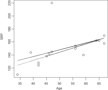
Figure 12.1 depicts systolic blood pressure as a function of age. Each circle corresponds to a pair of observations on a single individual. The solid line is the LAD regression line. The dotted line is the OLS regression line. A single individual, a 47 year-old with a systolic blood pressure of 220, is responsible for the difference between the two lines. Which line do you feel it would be better to use for prediction purposes?
FIGURE 12.1. Systolic blood pressure as a function of age LAD fit (solid line) and OLS fit (dotted line).

Opinions differ as to whether LAD is unstable in the sense that a small change in the data can cause a relatively large change in the fitted plane. Ellis [1998] reports that a change in the value of one observation by as little as 1/20,000th of the interquartile range of the predictor can result in a marked change in the slope of the LAD line.
Portnoy and Mizera [1998] strongly disagree and our own investigations support their thesis. The entire discussion may be viewed at http://projecteuclid.org/DPubS/Repository/1.0/Disseminate?view=body&id=pdf_1&handle=euclid.ss/1028905829.
The need for errors-in-variables (EIV) or Deming regression is best illustrated by the struggles of a small medical device firm to bring its product to market. First, they must convince regulators that their long-lasting device provides results equivalent to those of a less-efficient device already on the market. In other words, they need to show that the values V recorded by their device bears a linear relation to the values W recorded by their competitor, that is, that E(V) = a + bW.
But the errors inherent in measuring W (the so-called predictor) are as large if not larger than the variation inherent in the output V of the new device. The EIV regression method used to demonstrate equivalence differs in two respects from that of OLS:
Unfortunately, in cases involving only single measurements by each method, the ratio λ may be unknown and is often assigned a default value of one. In a simulated comparison of two electrolyte methods, Linnet [1998] found that misspecification of λ produced a bias that amounted to two-thirds of the maximum bias of the ordinary least-squares regression method. Standard errors and the results of hypothesis testing also became misleading. In a simulated comparison of two glucose methods, Linnet found that a misspecified error ratio resulted only in a negligible bias. Given a short range of values in relation to the measurement errors, it is important that λ is correctly estimated either from duplicate sets of measurements or, in the case of single measurement sets, specified from quality-control data. Even with a misspecified error ratio, Linnet found that Deming regression analysis is likely to perform better than least-squares regression analysis.

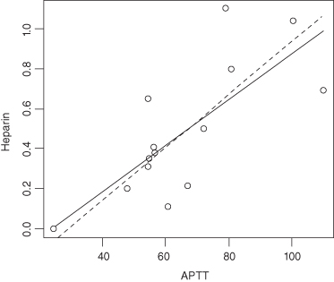
FIGURE 12.2. Solid line is OLS, Dashed line is EIV. λ = 1600.

In practice, Stöckl, Dewitte, and Thienpont [1998] find that it is not the statistical model but the quality of the analytical input data that is crucial for interpretation of method comparison studies.
Perfect correlation (ρ2 = 1) does not imply that two variables are identical but rather that one of them, Y, say, can be written as a linear function of the other, Y = a + bX, where b is the slope of the regression line and a is the intercept.
In method comparison studies, we need to be sure that differences of medical importance are detected. As discussed in Chapter 2, for a given difference, the necessary number of samples depends on the range of values and the analytical standard deviations of the methods involved.
Linnet [1999] finds that the sample sizes of 40–100 conventionally used in method comparison studies often are inadequate. A main factor is the range of values, which should be as wide as possible for the given analyte. For a range ratio (maximum value divided by minimum value) of 2, 544 samples are required to detect one standardized slope deviation; the number of required samples decreases to 64 at a range ratio of 10 (proportional analytical error). For electrolytes having very narrow ranges of values, very large sample sizes usually are necessary. In case of proportional analytical error, application of a weighted approach is important to assure an efficient analysis; for example, for a range ratio of 10, the weighted approach reduces the requirement of samples by more than 50%.
Linear regression techniques (OLS, LAD, or EIV) are designed to help us predict expected values, as in E(Y) = μ + βX. But what if our real interest is in predicting extreme values, if, for example, we would like to characterize the observations of Y that are likely to lie in the upper and lower tails of Y’s distribution. This would certainly be the case for economists and welfare workers who want to predict the number of individuals whose incomes will place them below the poverty line, physicians, bacteriologists, and public health officers who want to estimate the proportion of bacteria that will remain untouched by various doses of an antibiotic; ecologists and nature lovers who want to estimate the number of species that might perish in a toxic waste spill, and industrialists and retailers who want to know what proportion of the population might be interested in and can afford their new product.
In estimating the τth quantile,1 we try to find that value of β for which Σkρτ(yk − f[xk,β]) is a minimum, where

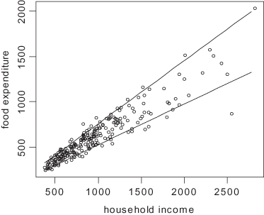
Even when expected values or medians lie along a straight line, other quantiles may follow a curved path. Koenker and Hallock applied the method of quantile regression to data taken from Ernst Engel’s study in 1857 of the dependence of households’ food expenditure on household income. As Figure 12.3 reveals, not only was an increase in food expenditures observed as expected when household income was increased, but the dispersion of the expenditures increased also.
FIGURE 12.3. Engel data with quantile regression lines superimposed.

Some precautions are necessary. As Brian Cade notes, the most common errors associated with quantile regression include:
Survival analysis is used to assess time-to-event data including time to recovery and time to revision.
Most contemporary survival analysis is built around the Cox model for which the hazard function takes the form  , where for each observation
  is a 1 × p row vector of covariate values and
  is a p × 1 column vector of to-be-estimated coefficients. Possible sources of error in the application of this model include all of the following:
Therneau and Grambsch [2000] cite the example of a heterogeneous population, 40% of whom acquire an infection at a rate of once per year and respond to a drug approximately half the time, 40% of whom acquire an infection at a rate of twice per year and respond to a drug approximately half the time, and 20% of whom acquire the infection as often as ten times per year and respond to the drug only 20% of the time. Let us launch a study with 1000 individuals in each treatment arm. Assuming that the infections follow a simple Poisson process, the expected number of individuals who will finish the year with k = 1, 2, … infections is given in the following table:

Clearly, in this example the treatment helps reduce the number of infected individuals. But does it reduce the number of infections? You will need to construct a table for your own data similar to the one above before you can be sure whether the heterogeneity of individuals’ susceptibility plays a role.
The Court wrote in NAACP v. City Of Niagara Falls, “Simple regression does not allow for the effects of racial differences in voter turnout; it assumes that turnout rates between racial groups are the same.”2 Whenever distinct strata exist, one ought develop separate regression models for each stratum. Failure to do so constitutes the ecological fallacy.
In the 2004 election for Governor of the State of Washington, out of the over 2.8 million votes counted, just 261 votes separated the two leading candidates, Christine Gregoire and Dino Rossi, with Mr. Rossi in the lead. Two recounts later, Ms. Gregoire was found to be ahead by 129 votes. There were many problems with the balloting, including the discovery that some 647 felons voted despite having lost the right to vote. Borders et al. v. King County et al. represents an attempt to overturn the results, arguing that if the illegal votes were deducted from each precinct proportional to the relative number of votes cast for each candidate, Mr. Rossi would have won the election.
The Court finds that the method of proportionate deduction and the assumption relied upon by Professors Gill and Katz are a scientifically unaccepted use of the method of ecological inference. In particular, Professors Gill and Katz committed what is referred to as the ecological fallacy in making inferences about a particular individual’s voting behavior using only information about the average behavior of groups; in this case, voters assigned to a particular precinct. The ecological fallacy leads to erroneous and misleading results. Election results vary significantly from one similar precinct to another, from one election to another in the same precinct, and among different candidates of the same party in the same precinct. Felons and others who vote illegally are not necessarily the same as others in the precinct.
… [T]he Court finds that the statistical methods used in the reports of Professors Gill and Katz ignore other significant factors in determining how a person is likely to vote. In this case, in light of the candidates, gender may be as significant or a more significant factor than others. The illegal voters were disproportionately male and less likely to have voted for the female candidate.3
To see how stratified regression would be applied in practice, consider a suit4 to compel redistricting to create a majority Hispanic district in Los Angeles County. The plaintiffs offered in evidence two regression equations to demonstrate differences in the voting behavior of Hispanics and non-Hispanics:

where Yhi and Yti are the predicted proportions of voters in the ith precinct for the Hispanic candidate and for all candidates, respectively; Ch and Ct are the percentages of non-Hispanic voters who voted for the Hispanic candidate or any candidate; bh and bt are the added percentages of Hispanic voters who voted for the Hispanic candidate or any candidate; Xhi is the percentage of registered voters in the ith precinct who are Hispanic; and εhi and εti are random or otherwise unexplained fluctuations.
If there were no differences in the voting behavior of Hispanics and non-Hispanics, then we would expect our estimates of bh and bt to be close to zero. Instead, the plaintiffs showed that the best fit to the data was provided by the equations


Of course, other estimates of the Cs and bs are possible, as only the Xs and Ys are known with certainty. It is conceivable, though unlikely, that few if any of the Hispanics actually voted for the Hispanic candidate.
Nonlinear regression methods are appropriate when the form of the nonlinear model is known in advance. For example, a typical pharmacological model will have the form A exp[bX] + C exp[dW]. The presence of numerous locally optimal but globally suboptimal solutions creates challenges, and validation is essential. See, for example, Gallant [1987] and Carroll et al. [1995].
To be avoided are a recent spate of proprietary algorithms available solely in software form that guarantee to find a best-fitting solution. In the words of John von Neumann, “With four parameters I can fit an elephant and with five I can make him wiggle his trunk.” Goodness of fit is no guarantee of predictive success, a topic we take up repeatedly in subsequent chapters.
Use a graph to report the results of a univariate regression only if one of the following is true:
Confidence limits should not be parallel; rather, they will appear hyperbolic around a regression line, reflecting the greater uncertainty at the extremes of the distribution.
In this chapter, we distinguished linear from nonlinear regression and described a number of alternatives to ordinary least squares regression, including least absolute deviation regression, and quantile regression. We also noted the importance of using separate regression equations for each identifiable stratum.
Consider using LAD regression when analyzing software data sets [Miyazaki et al., 1994] or meteorological data [Mielke et al., 1996], but heed the caveats noted by Ellis [1998].
Only iteratively reweighed general Deming regression produces statistically unbiased estimates of systematic bias and reliable confidence intervals of bias. For details of the recommended technique, see Martin [2000].
Mielke and Berry [2001, Section 5.4] provide a comparison of MRPP, Cade–Richards, and OLS regression methods. Stöckl, Dewitte, and Thierpont [1998] compare ordinary linear regression, Deming regression, standardized principal component analysis, and Passing–Bablok regression.
For more on quantile regression, download Blossom and its accompanying manual from http://www.fort.usgs.gov/products/software/blossom/.
For R code to implement any of the preceding techniques, see Good [2005, 2012].
Notes
* Y|X is read as Y given X.
1 τ is pronounced tau.
2 65 F.3d 1002, n2 (2nd Cir. 1994).
3 Quotations are from a transcript of the decision by Chelan County Superior Court Judge John Bridges, June 6, 2005.
4 Garza et al v. County of Los Angeles, 918 F.2d 763 (9th Cir), cert. denied.