If you measure n variables (each of a different type) of a single object, then you get a table with n columns for each object row. If there are m observations, then we have m rows of data. For example, given the student grades as data, you might want to know compute the average grade for each socioeconomic group, where grade and socioeconomic group are both columns in the table, and there is one row per student.
DataFrame is the most natural representation to work with such a (m x n) table of data. They are similar to Pandas DataFrames in Python or data.frame in R. DataFrame is a more specialized tool than a normal array for working with tabular and statistical data, and it is defined in the DataFrames package, a popular Julia library for statistical work. Install it in your environment by typing in add DataFrames in the REPL. Then, import it into your current workspace with using DataFrames. Do the same for the DataArrays and RDatasets packages (which contain a collection of example datasets mostly used in the R literature).
A common case in statistical data is that data values can be missing (the information is not known). The Missings package provides us with a unique value, missing, which represents a non-existing value, and has the Missing type. The result of the computations that contain the missing values mostly cannot be determined, for example, 42 + missing returns missing.
DataFrame is a kind of in-memory database, versatile in the various ways you can work with data. It consists of columns with names such as Col1, Col2, and Col3. All of these columns are DataArrays that have their own type, and the data they contain can be referred to by the column names as well, so we have substantially more forms of indexing. Unlike two-dimensional arrays, columns in DataFrame can be of different types. One column might, for instance, contain the names of students and should therefore be a string. Another column could contain their age and should be an integer.
We construct DataFrame from the program data as follows:
// code in Chapter 8\dataframes.jl
using DataFrames, Missings
# constructing a DataFrame:
df = DataFrame()
df[:Col1] = 1:4
df[:Col2] = [exp(1), pi, sqrt(2), 42]
df[:Col3] = [true, false, true, false]
show(df)
Notice that the column headers are used as symbols. This returns the following 4 x 3 DataFrame object:

show(df) produces a nicely formatted output (whereas show(:Col2) does not). This is because there is a show() routine defined in the package for the entire contents of DataFrame.
We could also have used the full constructor, as follows:
df = DataFrame(Col1 = 1:4, Col2 = [e, pi, sqrt(2), 42],
     Col3 = [true, false, true, false])
You can refer to columns either by an index (the column number) or by a name; both of the following expressions return the same output:
show(df[2])
show(df[:Col2])
This gives the following output:
[2.718281828459045, 3.141592653589793, 1.4142135623730951,42.0]
To show the rows or subsets of rows and columns, use the familiar splice (:) syntax, for example:
- To get the first row, execute df[1, :]. This returns 1x3 DataFrame:
| Row | Col1 | Col2    | Col3 |
|-----|------|---------|------|
| 1   | 1    | 2.71828 | true |
- To get the second and third row, execute df [2:3, :].
- To get only the second column from the previous result, execute df[2:3, :Col2]. This returns [3.141592653589793, 1.4142135623730951].
- To get the second and third columns from the second and third row, execute df[2:3, [:Col2, :Col3]], which returns the following output:
2x2 DataFrame
 | Row | Col2    | Col3  |
 |---- |-----   -|-------|
 | 1   | 3.14159 | false |
 | 2   | 1.41421 | true  |
The following functions are very useful when working with DataFrames:
- The head(df) and tail(df) functions show you the first six and the last six lines of data, respectively. You can see this in the following example:
df0 = DataFrame(i = 1:10, x = rand(10),
                y = rand(["a", "b",  "c"], 10))
head(df0
- The names function gives the names of the names(df) columns. It returns 3-element Array{Symbol,1}: :Col1 :Col2 :Col3.
- The eltypes function gives the data types of the eltypes(df) columns. It gives the output as 3-element Array{Type{T<:Top},1}: Int64 Float64 Bool.
- The describe function tries to give some useful summary information about the data in the columns, depending on the type. For example, describe(df) gives for column 2 (which is numeric) the minimum, maximum, median, mean, number of unique, and the number of missing:

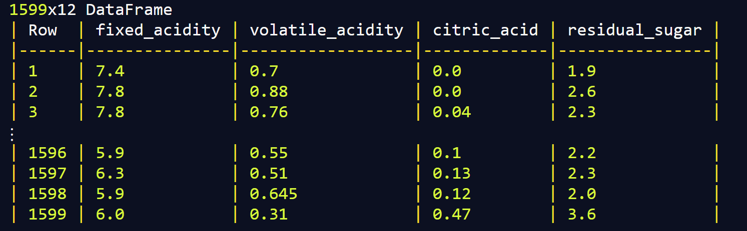
To load in data from a local CSV file, use the read method from the CSV package (the following are the docs for that package: https://juliadata.github.io/CSV.jl/stable/). The returned object is of the DataFrame type:
// code in Chapter 8\dataframes.jl
using DataFrames, CSV
fname = "winequality.csv"
data = CSV.read(fname, delim = ';')
typeof(data) # DataFrame
size(data) # (1599,12)
Here is a fraction of the output:
The readtable method also supports reading in the gzip CSV files.
Writing DataFrame to a file can be done with the CSV.write function, which takes the filename and DataFrame as arguments, for example, CSV.write ("dataframe1.csv", df, delim = ';'). By default, write will use the delimiter specified by the filename extension and write the column names as headers.
Both read and write support numerous options for special cases. Refer to the docs for more information.
To demonstrate some of the power of DataFrames, here are some queries you can do:
- Make a vector with only quality information, data[:quality].
- Give wines whose alcohol percentage is equal to 9.5, for example, data[ data[:alcohol] .== 9.5, :].
Here, we use the .== operator, which does an element-wise comparison. data[:alcohol] .== 9.5 returns an array of Boolean values (true for datapoints, where :alcohol is 9.5, and false otherwise). data[boolean_array, : ] selects those rows where boolean_array is true.
- Count the number of wines grouped by quality with by(data, :quality, data -> size(data, 1)), which returns the following:
6x2 DataFrame
| Row | quality | x1  |
|-----|---------|-----|
| 1    | 3      | 10  |
| 2    | 4      | 53  |
| 3    | 5      | 681 |
| 4    | 6      | 638 |
| 5    | 7      | 199 |
| 6    | 8      | 18  |
- The DataFrames package contains the by function, which takes in three arguments:
- DataFrame, here it takes data
- A column to split DataFrame on, here it takes quality
- A function or an expression to apply to each subset of DataFrame, here data -> size(data, 1), which gives us the number of wines for each quality value
Another easy way to get the distribution among quality is to execute the histogram hist function, hist(data[:quality]), which gives the counts over the range of quality (2.0:1.0:8.0,[10,53,681,638,199,18]). More precisely, this is a tuple with the first element corresponding to the edges of the histogram bins, and the second denoting the number of items in each bin. So there are, for example, 10 wines with quality between 2 and 3.
To extract the counts as a count variable of the Vector type, we can execute _, count = hist(data[:quality]); _; this means that we neglect the first element of the tuple. To obtain the quality classes as a DataArray class, we execute the following:
class = sort(unique(data[:quality]))
We can now construct df_quality, a DataFrame type with class and count columns as df_quality = DataFrame(qual=class, no=count). This gives the following output:
6x2 DataFrame
| Row | qual | no  |
|-----|------|-----|
| 1   | 3    | 10  |
| 2   | 4    | 53  |
| 3   | 5    | 681 |
| 4   | 6    | 638 |
| 5   | 7    | 199 |
| 6   | 8    | 18  |
To deepen your understanding and learn about the other features of Julia's DataFrames (such as joining, reshaping, and sorting), refer to the documentation available at http://juliadata.github.io/DataFrames.jl/latest/index.html.