2
Fundamentals of Commodity Economics: Supply
As with other tradable economic goods, there is a market for commodities that brings together supply from producers and demand from consumers. According to standard economic theory, producers attempt to maximize profits by adjusting economic decisions within the production constraints of resource inputs and technological feasibility. Consumers attempt to maximize utility from consumption within the constraints of their budget. The relationship between supply and demand is represented graphically in the price-quantity space by a downward-sloping demand curve between quantity and price and an upward-sloping supply curve between quantity and price. Equilibrium is achieved where the two curves intersect at the market-clearing price and quantity. The price of the commodity is the key economic variable that links supply and demand.
This chapter focuses on the supply side of commodity markets, in particular reviewing the major economic dynamics behind the production and supply of oil, the most heavily traded (and heavily studied) of energy commodities.
We will discuss three major models or frameworks that attempt to reflect observed trends in energy supply. These are Hotelling’s model, Hubbert’s Peak, and industry supply curves. Although all three have their flaws, each captures important realities of energy supply, which explains their popularity and longevity. But only through understanding all three would a student be able to develop a more holistic picture of energy supply dynamics.
Hotelling’s Model: Optimal Production with a Nonrenewable Resource
We begin with the famous model developed in 1931 by the American economist Harold Hotelling (1895–1973), which has become a workhorse of standard textbook treatments of resource economics.1 In its simplest form, Hotelling considered the economics of a single mine, making significant assumptions on the way. His main theoretical intention was to demonstrate that the equilibrium resulting from a price-taking firm operating the mine under competitive markets achieved a socially optimal outcome. A more detailed mathematical exposition of Hotelling’s model and the optimal control theory to solve it is provided in Mathematical Appendix A at the end of this chapter. Here we concentrate on understanding the intuition.
A Simple Two-Period Hotelling Model
Hotelling considered a mine owner who is trying to optimize the supply of resources extracted from a single mine, which is imagined as a single large and known block of mineral or pool of oil. (Some economists have likened it to a simple “cake” to be divided and eaten.)
Hotelling made a number of assumptions to simply his model. These include the following:
- 1. The amount of commodity in the mine is known and fixed.
- 2. The commodity is perfectly homogeneous and it takes a constant marginal cost to extract each unit of the commodity.
- 3. The producer (or mine operator) has perfect levels of control over the rate of extraction.
- 4. The quantity demanded for the commodity is a simple downward-sloping linear function with respect to price.
- 5. There is a single and constant interest rate on capital set by markets.
Hotelling’s model has been applied to try to explain mine production or even global supply for an exhaustible resource, but the logic and assumptions probably makes more sense for the operator of an amount of stored inventory.
For the sake of simplicity, suppose the mine is a well containing just two gallons of oil. The producer has two days to extract the oil, and it costs $1 to extract each gallon. He faces a simple linear demand curve, with price  each day.
In other words, if the supply on any day is two gallons, the price will be $2 (= 4 – 2) per gallon. If the supply is one gallon, the price is $3 (= 4 – 3) per gallon, and if there is no supply, the price buyers would be willing to pay is $4 (= 4 – 0) per gallon. Also, let’s assume the oil producer faces an interest rate of 10% per day. (This is all highly stylized but it makes the arithmetic easy!)
At its core, Hotelling’s model is about intertemporal optimization. The producer has to decide how much to extract each day. Let’s call the amount of oil he extracts the first day (today) q0 and the second day q1. It would be wasteful to have any oil left at the end of two days, so obviously, q0 + q1 = 2. What should the producer do?
He could take out all two gallons of the oil today, that is, set q0 = 2, q1 = 0. But that means he will be dumping two gallons of oil onto the market on the first day at the price of only p0 = 4 − 2 = $2 per gallon, depressing the market price, while leaving nothing for tomorrow, when prices p1 = 4 − 0 = $4 will be higher because of scarcity. The owner’s profit would be the $2 per barrel sale price minus the $1 per barrel cost, or a $1 profit on the two gallons sold today (and none tomorrow), or $2 profit total. Maybe the producer should have waited to produce tomorrow when prices will be higher.
But if he produced nothing today and everything tomorrow, then the same thing will happen. Prices today surge to $4 because of scarcity and depress to $2 tomorrow, leaving the same $2 in total profit. To add insult to injury, the profit would only come on the second day, forcing the producer to wait an extra day to see the $2 profit.
Suppose the owner sets production at one gallon each day. This is more promising. Then prices will be $3 every day, or a $2 profit on each gallon sold, $1 each from the gallon sold today and tomorrow. This means the producer would earn a profit of $2 today and another $2 tomorrow. This is certainly better than the strategy of producing everything on the first day or the second day!
But this still isn’t perfect. After all, there is the time value of money. The interest rate is 10% per day. If the miner produces a little bit more on the first day, he may be able to earn a little extra by taking that extra revenue, putting it into a bank, and earning interest over that day rather than waiting to earn that profit tomorrow.
Hotelling’s insight is about how to perfectly optimize between these two periods. Economists always consider optimization at the margin. Consider the last marginal drop of oil producible from the well after dividing the remaining two barrels evenly between the two days. Should the owner produce it today or tomorrow?
If he produces it today, he’ll get a $2 per gallon profit on that drop today. If he saves it for tomorrow, he’ll reap a $2 per gallon profit on that drop tomorrow. But these amounts do not produce the same profit. Because of interest, the $2 profit per barrel tomorrow is closer to $1.82 in profit today once the $2 is discounted by 10%. So it is better to produce that drop today and get $2 in profit today than get $1.82 tomorrow. But the same will be true of the next drop, and the next drop after that, until the producer finds that more production today is depressing prices and his profits today while boosting prices tomorrow.
Hotelling argued that the producer should extract just the right amount of oil each day to make the producer indifferent between today and tomorrow. What is the right price and quantity level that would make the producer indifferent? Well, since time is money, his profit per barrel in nominal terms should also be increasing at the rate of interest.
In other words, the profit per barrel, often denoted as  , should satisfy the following equation:
  . This is the only way the producer is completely indifferent between today and tomorrow and maximizes the present value of his total profits. It turns out that producing q0 = 1.1 and q1 = 0.9 is about the right balance between not overproducing too much in the first day yet biasing toward earlier production because of the time value of money.
The intuition that  , also known as the economic rent or the shadow price from the well, must be rising at the rate of interest is famously known as “Hotelling’s Rule.”
A Multiperiod Example
Let’s step up the complexity one notch and consider a multiperiod example of ten years. Suppose that the oil field now has a more realistic 292 million barrels of oil, and that you are able to produce at marginal costs equal to c = $10 per barrel. With an inverse demand equation of  , and a discount rate of r = 10% per annum, what would the optimal production profile be?
Using the same intuition as above, Hotelling’s Rule states that economic rent, which is again prices minus costs, should be rising at the rate of interest:  , where
  .
.
Inserting the prices going backward for every individual period, we use the equation to find the quantity extracted in the earlier periods until we reach the very beginning. (See table 2.1 and figure 2.1 for a better illustration.)
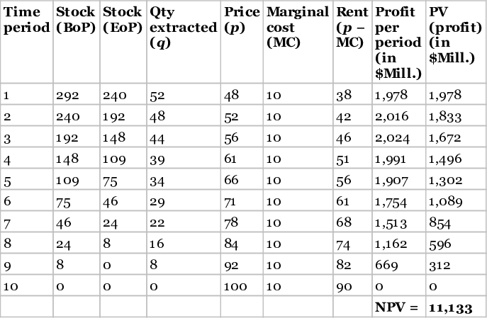
Note: BoP, beginning of period; EoP, end of period; PV, present value; NPV, net present value.
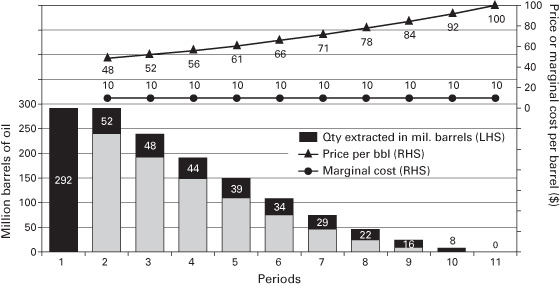
Figure 2.1 Multiperiod Hotelling model simulation.
The value of the resource extracted today must equal the discounted value of the resource extracted in the future, or else there is suboptimal extraction. In other words, the shadow value of the resource must be rising exponentially at the discount rate.
Why should the shadow price be increasing at the rate of interest? The reason to delay extraction of a resource is the presence of a discount rate. As such, an optimizing agent will delay the extraction of a resource only when the appreciation in the value of the capital (in this case the oil itself) compensates for the loss suffered in terms of time lost from not producing today.
A Continuous-Time Approach to Hotelling’s Model
Having explored the intuition of Hotelling using discrete-time examples, we now continue our discussion using a continuous-time mathematical model (similar to that used in Hotelling’s original paper) to investigate the ways theorists have tried to modify and extend Hotelling’s framework. The Mathematical Appendix A provides the full derivation, but to quickly sketch the basic framework, Hotelling considered competitive firms maximizing the discounted value of the stream of profit:
where  is the price at time t,
  is the quantity extracted at time t,
  is the marginal cost of extraction, and
  is the discount rate.
From the appendix, we have Hotelling’s rule in continuous-time form:
The economic rent  from the resource, that is, the price minus the cost, still grows exponentially at the discount rate (See figure 2.2). Note, however, in the competitive market case, the discount rate is the market rate of interest.
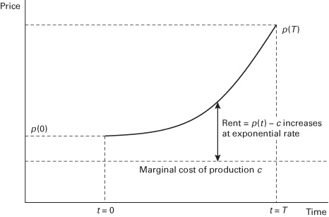
Figure 2.2 Hotelling’s rule of exponential growth.
It is important to recognize the “fragility” of Hotelling’s model. If prices deviate even slightly from Hotelling’s rule of exponential growth at the discount rate, then producers should immediately race to produce in order to exploit that deviation and extract the entire mine all at once, since there is no cost of adjustment or storage.
Relaxing Hotelling’s Assumptions
Hotelling provides an elegant analytical framework incorporating an important insight into the economics of supply, namely, that of intertemporal optimization. But as we shall see in the next chapter, in practice, many commodity prices seem stationary in the long run; that is, they don’t seem to have a clear upward trend. This seemingly conflicts with Hotelling’s rule, which predicts exponentially increasing commodity rents (and therefore, after adjusting for costs, prices). In this section we try to relax some of the assumptions in Hotelling’s model and see if it helps give more real-world applicability.
Backstop Technology
One simple way to extend the model is to consider possible substitutes for the resource. When the price of extracting a resource becomes equal to or higher than that of a substitute, the substitute is likely to replace that resource in the economy. For example, if the price of fossil fuels becomes too high, people might switch to alternative energy sources as a “backstop,” such fusion power or other energy sources. One can also consider backstop technologies as simply a cheaper substitute, such as cheaper natural gas replacing coal. But the important assumption is that once the switch to a backstop technology is made, there is no going back. The investment into the backstop technology is irreversible (a point we will return to in chapter 6 on real options).
A backstop technology can only be feasibly employed in the extraction process once the price of the resource becomes high enough to justify a transition out of it and into the substitute technology. Accordingly, the payoff function for resource extraction must take into account the cost  associated with the use of a backstop technology, where
  in order for resource extraction to take place using the original technology. As long as the shadow price plus marginal cost is lower than that of the backstop technology, no transition to the backstop technology will take place.
If we consider an exogenous backstop technology b, the instantaneous payoff function would change to:
where  is the cost of the backstop technology, which is unconstrained in its use:
As long as  , then the usage of backstop technology
  . Once
  , however, producers will switch to the backstop technology. There will be an exponential rise in shadow prices until
  , as shown in figure 2.3. This is a rather boring extension of Hotelling but does remind us that consumers may face substitutes beyond the resource itself.
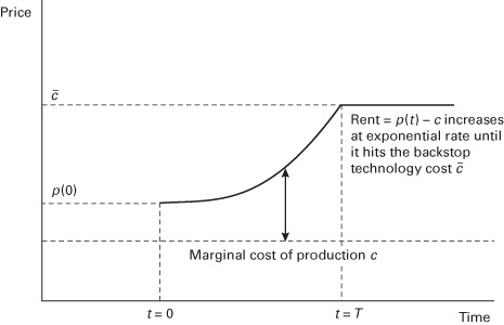
Figure 2.3 Hotelling’s rule with a backstop technology.
In practice, however, substitutes are likely going through their own complex supply-and-demand dynamics, and a switch to an alternative (e.g., from gasoline-powered to electric vehicles) is not costless and simple. Furthermore, the development of substitutes is likely itself to depend on the price of the resource, as a higher resource price incentivizes the search for alternatives.
Variable Mine Quality
Owing to numerous geological, geopolitical, and technological conditions, resource mines may not have uniform qualities and extraction costs. For example, onshore oil fields in the Middle East may have extraction costs as low as $10 per barrel, while the oil sands in Canada often break even around $80 to $100 per barrel. How can this reality of variable mine qualities be factored into Hotelling’s model?
Consider a firm that owns two mines with different marginal costs of extraction, c1 and c2. It can be shown that the firm will choose to not exploit two mines of different qualities simultaneously. Rather, the firm will opt to deplete the cheaper mine first, with the rent increasing exponentially as per the usual rule until it hits the point where the producer finds it more efficient to move on to the other mine. This intermediate time of switching occurs when the economic rent from the first mine exactly equals the rent from the second mine:
Figure 2.4 shows how once the switch to the second, more expensive mine is made, the same Hotelling’s rule dynamic holds again, now at the higher marginal cost of production.
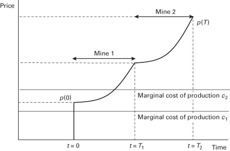
Figure 2.4 Two heterogeneous mines, illustrating dynamic of Hotelling’s rule twice.
In practice, there are many reasons why this framework is still too simplistic. Resource producers may face capacity constraints that prevent full and cost-effective extraction from the first mine even if it is cheaper to do so. For example, too rapid extraction from an oil field can damage it by causing its geological pressure to drop too quickly, reducing the amount of oil ultimately recoverable from the field and its long-term value. Hotelling’s assumption that firms have fine-tuned control over the extraction rate is an extreme one when producers face numerous short-term geological, technological, and financial constraints.
In the medium and long term, however, firms do have better control over the investment decisions that ultimately determine the rate of extraction. In fact, the recent breakthrough in using horizontal hydraulic fracturing technologies to extract from shale oil basins has given oil companies better control over their production output because the decline rate from fracking wells is much steeper and production is much more closely linked to a firm’s drilling decisions.
Market Power
Hotelling’s model assumes that markets for the extracted resource are perfectly competitive and that firms maximize their extraction rates as price-takers. In reality, some producers may have the market power to affect prices directly, and Hotelling’s model can be modified accordingly. Instead of a price-taking small firm, let’s consider a monopolist facing a demand curve. The payoff function becomes:
This looks almost identical to the competitive market case, but importantly, the monopolist now considers how his production decisions affect prices in maximizing his profit.
In this case, the first-order condition (FOC) becomes:
Since the demand function is downward sloping in quantity, the derivative is negative and extraction proceeds at a slower rate than under competitive markets, as the price-setting monopolist adjusts production in order to maximize profits. Box 2.1 goes into more detail on the role of the Organization of Petroleum Exporting Countries or OPEC in monopolistic behavior in the oil market. But we still have from the second condition positing Hotelling’s rule of exponentially increasing economic rents.
Box 2.1
Hotelling and OPEC
Why does the world rely on a variety of relatively expensive oil suppliers from different basins rather than on the lowest-cost source of supply? In a competitive market, we would expect consumers to purchase from the lowest cost producer. However, nonrenewable markets do not operate this way. That’s because most major oil producers maintain monopolistic control over their oil and natural gas reserves through sovereign state-owned oil companies. Many of these national oil companies (NOCs) are also part of an international cartel, the Organization of Petroleum Exporting Companies or OPEC. These monopolistic producers coordinate their production to affect prices. (We discuss NOCs in more detail in chapter 9.) As a result, the members of this cartel are not price-takers but price-makers. The cartel evaluates the global demand curve and the way in which prices adjust to the quantity supplied. By keeping the quantity supplied below the level that would be supplied under perfectly competitive conditions, they artificially increase prices and therefore their ultimate profit. OPEC is a classic example of an oligopoly (though one that faces constant internal political tensions and challenges of enforcement).
Ironically, this allows other competitive firms in non-OPEC areas to produce and sell oil at higher prices than they otherwise would and remain profitable, since they don’t have to compete with ultra-cheap OPEC crude. Because OPEC members deliberately hold back quantities of supply, they aren’t driven out of the market. Here is yet another example where the elegant theory of Hotelling collides with the messy real world.
We covered various extensions to Hotelling’s original framework—the existence of alternative technological substitutes, the presence of variable mine qualities and costs, and price-making producers.
Yet two core assumptions remain: (1) that producers have perfect information about the amount of resource in their mines and the future trajectory of prices, and (2) that they have perfect control over the exact speed of extraction. It’s as if the mine were not a mine at all but a giant storage tank ready to release. Naturally, geologists and mining engineers would beg to differ!
It turns out that for most practical contexts, engineering challenges preventing fine-tuned extraction, a high degree of uncertainty about the future, and other economic, political, and technological constraints “swamp” the Hotelling effect of exponentially increasing economic rents.
Nonetheless, the model does capture an essential reality of natural resource extraction: that producers will strive to optimize production intertemporally and that the problem of resource extraction should be thought of as a dynamic problem, not a static one.
Hubbert: The Geologist’s Approach
Having completed our introduction to Hotelling’s model, we turn next to the model introduced by Marion King Hubbert (1903–1989). As we saw above, Hotelling largely ignores the geological and engineering challenges associated with finding and extracting the resource. Hubbert’s approach puts those challenges at the very center of his analysis. Hubbert, or “King Hubbert,” as he was known, was not an economist but an American geoscientist and engineer. Nevertheless, his model of a resource basin through a geological life cycle has proven very influential and surprisingly practical.2
Hubbert was inspired by logistical models used to model the ecological dynamics of animal population growth and decay in a Malthusian world of limited food supply. He argued that similar boom-and-bust life cycles can apply to the supply of resources. (Mathematical Appendix B at the end of this chapter provides the mathematical derivation of Hubbert’s logistical model.) For example, when exploration in a particular geological reserve begins, the rate of growth of cumulative output rises “almost” exponentially as sweet spots are discovered and engineers gain a better understanding of the geology. However, much as the population of animals begins to plateau and then reverses as the food supply runs out, eventually the reserve begins to be exhausted as cumulative production approaches the ultimately recoverable quantity of the resource.
In contrast to Hotelling, Hubbert was not trying to model a single mine. Hubbert acknowledged that each mine may be forced to follow some rigid output schedule according to the stipulations of geology and mine pressure. But Hubbert argued that in a large-enough geological area, a macroscopic pattern can be detected by aggregating the discoveries and exploitation of multiple mines. Logistical growth in production as engineers improved their understanding of the geology through exploration and discovery would eventually hit the limits of the overall amount of recoverable resources in the region.

Figure 2.5 Single mine production schedule.
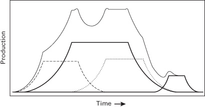
Figure 2.6 Aggregation of multiple mines.
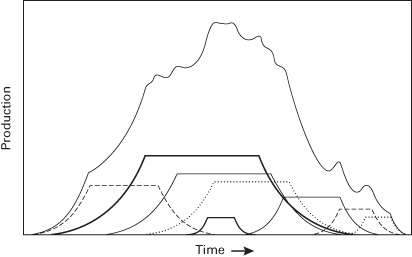
Figure 2.7 Emergence of Hubbert’s Logistical Bell Curve.
Figures 2.5 to 2.7 show how the aggregation of multiple smaller mines of various sizes and times of discovery eventually can create an overarching logistical bell curve.
Despite its simple and deterministic approach, Hubbert’s assumption turns out to be a fairly good fit for specific geological regions. The Hubbert model for Norway, for example, has thus far been a fairly accurate predictor of the country’s lifetime extraction path, insofar as Norway is its own geological region (figure 2.8).
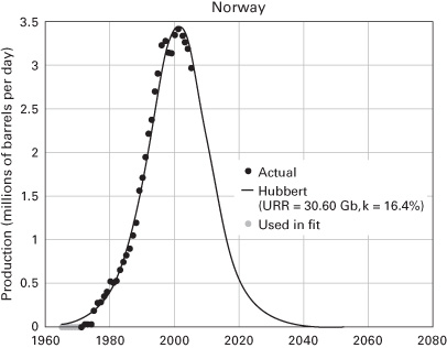
Figure 2.8 Hubbert’s bell curve for Norway.
However, when applied to a country like the United States, which is a much larger area with multiple geological regions, Hubbert’s model becomes relatively less precise. And most critically, as box 2.2 shows, Hubbert’s model contains no mechanism for taking into account advancing technology that may make new resource basins economical, or the fluctuations in prices that may incentivize slower or faster development of the basins in question.
Box 2.2
Hubbert’s Curve Broken: The U.S. Tight Oil Revolution
As shown in figure 2.9, U.S. oil production followed the path forecasted by Hubbert’s model reasonably closely throughout most of the twentieth century. Indeed, many analysts extrapolated from this extraction history to proclaim that “peak oil” in America was nigh and that production would inexorably decline subsequently. Yet beginning in the early 2010s, U.S. oil production diverged markedly from that predicted by Hubbert’s model. This was the result of the unconventional shale or “fracking” revolution, and it reveals much about the shortcomings of Hubbert’s model.
Apart from serious doubts as to whether Hubbert’s proposed aggregation is applicable beyond a single geological area, Hubbert’s aggregation flatly ignores economic forces driven by price dynamics and technological change.
The development of U.S. shale/tight oil was incentivized by higher prices, which spurred technological breakthroughs in combining hydraulic fracturing, horizontal drilling, and computer-aided seismic imaging that made previously known reserves of shale/tight oil economical. It opened up new reserves that were not in Hubbert’s initial parameterization, thus “breaking” Hubbert’s Peak Curve.
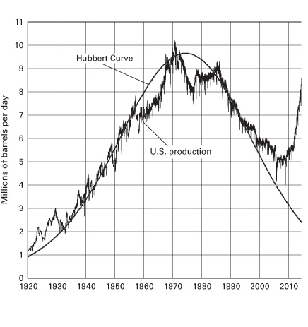
Figure 2.9 Hubbert’s curve broken: U.S. crude oil production vs. Hubbert’s curve. Jagged line indicates U.S. production (data source: U.S. Energy Information Administration); smooth curve denotes Hubbert’s bell curve. MMBPD, millions of barrels per day.
Peak Oil
When extrapolated to the entire world, Hubbert’s peak model seems to argue for a definite and predictable point of peak global supply of a nonrenewing resource like oil and eventual Malthusian catastrophe as the resource runs out. Here is where literal applications of Hubbert’s model have proved highly problematic.
Perhaps the most egregious mistake is in misunderstanding “technically recoverable” reserves as an exogenous geological estimate of the finite amount of resources left in the Earth’s crust. In fact, estimates of the amount of recoverable resources, despite being informed by geological characteristics, are economic variables strongly driven by price-based incentives to explore. In other words, as new technology makes more resources recoverable, the point at which we would say we have reached peak oil gets delayed. Hubbert’s model does not consider these endogenous economic considerations at all.
Figure 2.10 shows that in the case of oil, the technically recoverable amount of oil in the world has been steadily increasing despite the constant drain from consumption. Moreover, reserve estimates have increased faster in periods of high oil prices (as companies have become incentivized to search for more resources) and stagnate when oil prices are low.
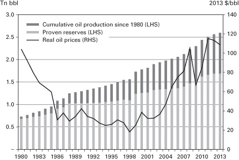
Figure 2.10 World Proven Reserves and Cumulative Production of Oil since 1980.
The concept of peak resource, by ignoring these economic dynamics, stands on shaky theoretical ground. Despite the appealing simplicity of a theory of peak resource that promises Malthusian catastrophe, economic forces and technological progress have trumped any exogenous constraints imposed by nature. It is worth quoting from Morris Adelman, a distinguished professor of energy economics at MIT, in full:
The assumption of an initial fixed stock is superfluous and wrong. Only a fraction of the mineral in the earth’s crust, or in any given field, will ever be used. … What we observe in the real world are not one-time stocks immaculately created to be consumed but inventories of “proved reserves,” constantly renewed by investment in finding and development. Over time, the investment needed per unit-added is forced up by diminishing returns, and forced down by increasing knowledge. So far, knowledge has prevailed.3
Hubbert’s model, while working well for studying the life cycle of a particular resource basin over relatively short periods of time when technologies and prices do not vary much, proves to be fatally flawed when extrapolated to world resource supply.
This is not surprising if you consider that while Hotelling focused on the question of optimization of a single mine, Hubbert instead focused on the life cycle of discovery and exhaustion under geological constraints while ignoring intertemporal optimization, or indeed, any economic considerations at all. Both models contain core “truths” but also make heroic assumptions that depart greatly from reality.
Industry Cost Curves
Analysts working in the industry often build cost curves in an attempt to summarize the quantities and total costs faced by heterogeneous regions across the world. This is done by stacking up the resource basins according to the amount of production they can achieve on one axis against the breakeven price at which developing the basin becomes economically attractive on the other axis. This seemingly creates a “supply” curve for a resource that compares quantity supplied with price required (figure 2.11).
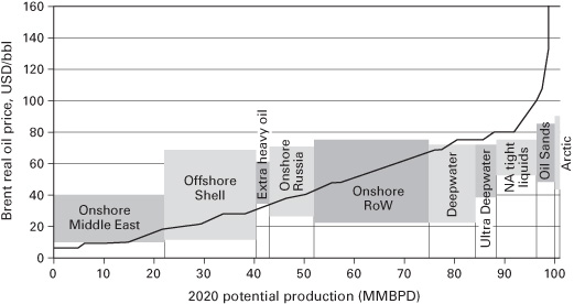
Figure 2.11 Cost of supply curve for global oil, 2020. Future oil prices will be determined by the marginal cost of developing new oil rather than by OPEC interventions. North American shale is expected to outcompete many oil sands and Arctic oil projects. MMBPD, million barrels per day.
Source: UCube by Rystad Energy.
Industry analysts like to argue that the price of the resource depends on the breakeven cost of that resource basin providing that last marginal unit of resource to meet demand. If prices rise, the next most economical basin would become economical and begin supplying the resource. Until then, it is turned “off.” This tacitly assumes that producers myopically produce the moment a price exceeds the breakeven cost and delivers minimum required rates of return on investment.
In contrast to Hotelling’s and Hubbert’s models, it is a bit of a stretch to call this last approach an actual model. Instead, it is more like an accounting of the various fixed and marginal costs faced by producers globally. The industry cost curves approach says nothing about how producers may accelerate or defer production depending on current and expected future prices. As we saw with Hotelling’s model, producers may defer production even when prices exceed costs if they know that prices may be even higher in the future. The industry cost curve approach assumes away intertemporal optimization and assumes that producers narrowly focus on immediate profit.
Like Hubbert’s model, the industry cost curve approach does acknowledge some of the geological aspects of supply determinants, captured in the differences in breakeven costs between basins. But the cost curve is purely static and, unlike Hubbert’s model, says nothing about the life cycle production profile over time.
Additionally, though the cost curve chart tries to summarize the total breakeven costs of production, it somewhat glosses over the fact that for many resource projects, producers face both the initial fixed costs of capital investment and the marginal but continuing costs of operation. Total breakeven costs capture the entire costs of both fixed and marginal costs. But in such circumstances, once a resource project is ready and the fixed cost is sunk, even when prices fall below the breakeven point, all production from existing projects that have already paid fixed costs will continue running as long as prices remain above the marginal costs of production. Hence it is somewhat misleading to imagine that resource basins will immediately “turn on” and “turn off” the moment prices exceed or fall below producers’ breakeven costs.
In summary, it can be said that the industry cost curves approach suggests a very static, myopic world. It takes into account geology and rational economic decision making but misses some of the key insights that are included in the other models. It might be better described as a useful accounting exercise that summarizes in one graph the menu of costs faced by potential producers.
Toward a New Theory of Supply
Hotelling’s model, Hubbert’s model, and the industry cost curves approach all manage to capture some aspects of the reality of the economics of resource supply today, but all also face significant limitations.
Hotelling’s central insight is that producers will attempt to optimize production of finite resources intertemporally. The theoretically elegant model can be extended to consider the relaxation of some assumptions, such as heterogeneous costs or market power. But crucially, Hotelling’s model relies heavily on the assumptions of perfect control over extraction rates and perfect information about prices, quantities, and costs. These ideal circumstances can be approximated under certain real-life scenarios, such as extraction of a resource from a single storage tank, and to a lesser extent shale fracking. However, Hotelling’s model fails to account for the real-life challenges of imperfect information and lack of fine-tuned production control. Hotelling’s starkest prediction—his famous rule that prices minus costs should rise exponentially at the discount rate—should not be taken so literally.
Hubbert’s logistical model for resource production proves surprisingly good at approximating the life cycle of exploration and development of a single geological basin, when prices are stable and all else remains constant. But when Hubbert’s curve is applied across long stretches of time or expanded from a single basin to multiple basins at a national or global scale, its lack of any modeling for economic or technological dynamics becomes increasingly problematic. Its most famous prediction, Hubbert’s peak, should also, like Hotelling’s rule, not be taken too literally.
Industry cost curves provide a useful snapshot of cost structures across different geological basins at any single point in time. However, this approach is quite static and glosses over important points of Hotelling and Hubbert. Industry cost curves ignore producer intertemporal optimization while considering the various production costs also analyzed by Hotelling, and the life cycle of exploration, development, and depletion analyzed by Hubbert.
All three models afford insight into a particular aspect of the economics of resource supply, but at the expense of abstracting from other complexities, they are in tension with each other. Hotelling’s model fails to account for the geological realities of resource extraction, a central tenet of Hubbert’s model, by assuming perfect information and perfect control over output. Hubbert’s curve features mines following rigid output schedules determined by their particular geology but does not take into account economic optimization or technological progress. Industry cost curves provide a useful static snapshot of diverse costs across various geological basins but feature neither dynamical optimization over time (as in Hotelling’s model) nor the geological life cycle (as in Hubbert’s model).
At the end of the day, analysts should embrace the insights afforded by each model while recognizing the shortcomings of all three approaches. Only by synthesizing the approaches and understanding when and under what circumstances each model is useful can one approach a more holistic understanding of the economic dynamics of commodity supply.
Mathematical Appendix A: Optimal Control Theory
Optimal control theory was developed in the 1950s and 1960s by Richard Bellman (1920–1984) in the United States and Lev Pontryagin (1908–1988) in the Soviet Union. Optimal control theory is an extension of the standard Lagrangian techniques utilized in the calculus of variations to solve various optimization problems.
In economics, when maximizing the discounted cash flows of a profit stream from an investment project, optimal control problems often take the form
where  is the payoff function,
  is the state variable,
  is the control variable, and
  is the discount rate. The state variable is controlled by the optimizer through the control variable and needs to follow a “law of motion”:
For example if  is the quantity of oil in the ground, then
  , the extraction rate. However,
  could also depend on
  itself. For example, such is the case in the optimal control of fisheries, where
  will result from both extraction
  and the amount of breeding, which itself depends on the size of the stock,
  .
.
Traditionally, we would define the Lagrangian as:
where  is known as the shadow price, which captures the incremental change in the objective function for every unit of change by which the constraint is relaxed or strengthened.
Using the Hamiltonian formulation, we have:
Intuitively,  can be thought of as the instantaneous payoff,
  is the shadow value of “capital” x, and g is the rate of change of capital
  . In other words, the term
  can be thought of as “capital appreciation” and the overall Hamiltonian is the instantaneous value creation at time t. The real underlying economic value of the investment project at any given point in time is the direct payoff the operator gets from the project plus some economic value that comes from increases or decreases in the capital stock according to how the investor is trying to control it:
Obtaining the following first-order conditions:
FOC 1 (optimization over control variable):
FOC 2 (no arbitrage condition):
The economic intuition behind this first-order condition is that if an investor has a unit of capital or stock worth  that could alternatively be invested in the bank at interest
  , the “profit” would be
  one period later. If instead the investor took the stock and put it into the optimal control problem to “do work,” it would increase the problem by one unit of x (i.e.,
  ). One period later the initial capital or stock could be resold for
  , yielding a “profit” of
To preclude arbitrage between these two investment options, and taking the limit as  , we must have:
When you consider a stock of oil in the ground for example, optimal control theory tells the investor that one need not have to worry about the complexities of the entire investment problem. The investor need only consider how to maximize the value gained from extracting oil (and getting a payoff from that) at each point in time balanced against the capital appreciation gain or loss associated with the fact that with every one barrel of oil extracted the investor loses the shadow value for the amount of oil in the ground. In this case, the shadow price could be thought of as the value of leasing rights.
Hotelling showed that the equilibrium resulting from price-taking firms owning a mine results in the same outcome as a social planner maximizing Marshallian consumer surplus, provided the interest rate used by the firm is equal to the social discount rate.
The problem of a social planner optimizing the output from a single mine, with constant marginal cost c, assuming the total stock of reserves in the mine is finite and known with perfect uncertainty, can be formulated this way:
where  is the welfare function, and the control variable
  is the extraction rate. The evolution of production is set by the function
  , where
  is the state variable (the amount of resource remaining in the mine at time t), which is pinned down by the collapsed transversality condition,
  .
.
The FOCs are derived as follows:
The second condition can be solved analytically:
The first condition shows that marginal welfare must equal the shadow price plus the marginal cost of extraction. The second condition shows that the shadow price changes exponentially at the discount rate  , famously known as Hotelling’s rule. It argues that the value of the resource extracted today must equal the discounted value of the resource extracted in the future, or else there is suboptimal extraction by the social planner.
For the competitive equilibrium case, we have firms maximizing profit:
The FOCs are derived as follows:
The economic rent from the resource still grows exponentially at the discount rate. Hence, Hotelling showed that the extraction speed of profit-seeking competitive firms replicates the optimization outcome of a social planner trying to optimize Marshallian consumer plus.
Hotelling’s insight is that if a company is extracting resources, it needs to think not just about immediate profits but intertemporally. Firms should consider how to maximize not just immediate profit but the whole value of the reserves, taking into account the entire trajectory of prices to the end of the life of the mine.
It should be noted that Hotelling’s rule applies to real inflation-adjusted prices, so in nominal terms, the economic rent should be rising at a slower rate of exponential growth or even be constant (if the real interest rate is zero).
Mathematical Appendix B: Hubbert’s Logistical Model
The American geologist M. King Hubbert assumed that the cumulative production from a geological area of reserves follows logistic growth:
where Q is the cumulative production, q is the instantaneous production, and k and  are constants.
The logistical growth model was developed by the Belgian mathematician Pierre François Verhulst (1804–1849) to model self-limiting population growth after Verhulst read the pessimistic assessment An Essay on the Principle of Population by the English economist Thomas Malthus (1766–1834).
Hubbert was motivated to follow Verhulst by the intuition that when exploration in a particular geological reserve first begins, the rate of growth of cumulative output rises “almost” exponentially as sweet spots are discovered and engineers gain a better understanding of the geology. However, much like the saturation capacity in a Malthusian world, eventually the reserve begins to exhaust itself as cumulative production approaches  , which is the ultimately recoverable quantity of reserves, and the rate of growth of cumulative production declines and reverses.
It is important to recognize that Hubbert was not trying to model a single mine. Each single mine may follow some rigid output schedule according to the dictates of geology and mine pressure, but after one aggregates the discoveries and exploitation of multiple mines in a large enough geological area and factors in the learning by doing versus the capacity of the area, the macroscopic pattern begins to mimic that of a logistical curve.
Hubbert’s model results in an ordinary differential equation that is easily solved:
Integrating on both sides, we get:
This is known as the logistical curve, or sigmoid function, which has a distinctive S shape.
The first derivative, or instantaneous production, creates a bell curve that looks similar to but is not the familiar Gaussian distribution. The Gaussian distribution has tails that decline at rate  , while the logistical bell curve declines at rate
  .
.
 ,
, .
. ,
, .
. .
. .
. .
. ,
, .
. ,
, .
. .
. .
. ,
, .
. .
. ,
, .
. ,
, ,
, .
. .
. .
.
 ,
, .
. ,
, ,
, ,
, .
.