Chapter 5. Data Modeling
The data model you use is the most important factor in your success with Cassandra.
Patrick McFadin
More than any configuration or tuning you can perform, your data model is the main factor that will affect your application performance and cluster maintenance. In this chapter, you’ll learn how to design data models for Cassandra, including a data modeling process and notation. To apply this knowledge, you’ll design the data model for a sample application, which you’ll build over the next several chapters. This will help show how all the parts fit together. Along the way, you’ll see some tools to help you manage your CQL scripts.
Conceptual Data Modeling
First, let’s create a simple domain model that is easy to understand in the relational world, and then see how you might map it from a relational to a distributed hash table model in Cassandra.
To create the example, we want to use something that is complex enough to show the various data structures and design patterns, but not something that will bog you down with details. Also, a domain that’s familiar to everyone will allow you to concentrate on how to work with Cassandra, not on what the application domain is all about.
Let’s use a domain that is easily understood and that everyone can relate to: making hotel reservations.
Our conceptual domain includes hotels, guests that stay in the hotels, a collection of rooms for each hotel, the rates and availability of those rooms, and a record of reservations booked for guests. Hotels typically also maintain a collection of “points of interest,” which are parks, museums, shopping galleries, monuments, or other places near the hotel that guests might want to visit during their stay. Both hotels and points of interest need to maintain geolocation data so that they can be found on maps for mashups, and to calculate distances.
The conceptual domain is shown in Figure 5-1 using the entity–relationship model popularized by Peter Chen. This simple diagram represents the entities in the domain with rectangles, and attributes of those entities with ovals. Attributes that represent unique identifiers for items are underlined. Relationships between entities are represented as diamonds, and the connectors between the relationship and each entity show the multiplicity of the connection.
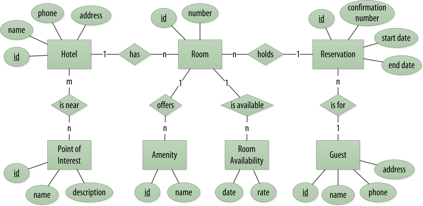
Figure 5-1. Hotel domain entity-relationship diagram
Obviously, in the real world, there would be many more considerations and much more complexity. For example, hotel rates are notoriously dynamic, and calculating them involves a wide array of factors. Here you’ll define something complex enough to be interesting and touch on the important points, but simple enough to maintain the focus on learning Cassandra.
RDBMS Design
When you set out to build a new data-driven application that will use a relational database, you might start by modeling the domain as a set of properly normalized tables and use foreign keys to reference related data in other tables.
Figure 5-2 shows how you might represent the data storage for an application using a relational database model. The relational model includes a couple of “join” tables in order to realize the many-to-many relationships from the conceptual model of hotels-to-points of interest, rooms-to-amenities, rooms-to-availability, and guests-to-rooms (via a reservation).
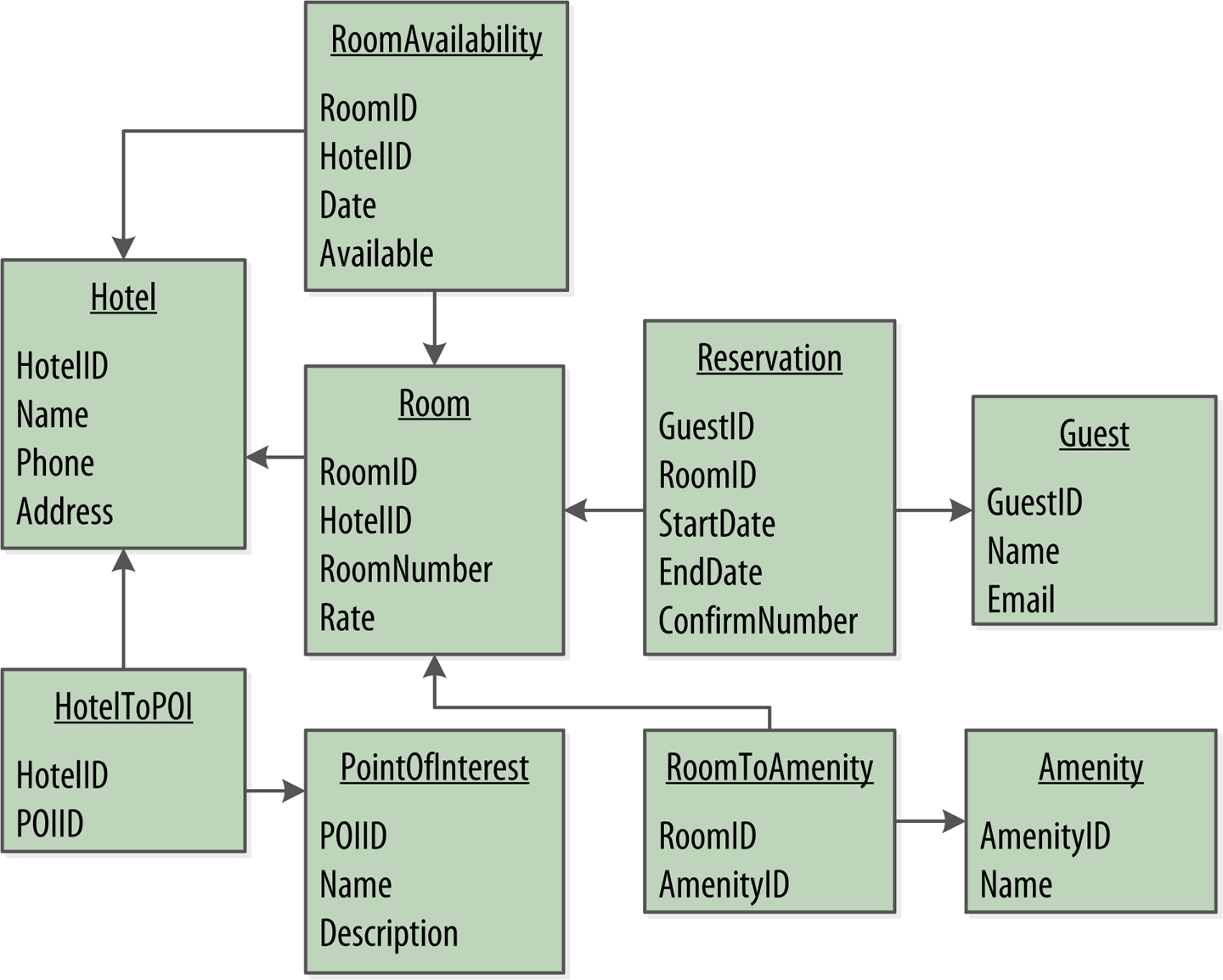
Figure 5-2. A simple hotel search system using RDBMS
Design Differences Between RDBMS and Cassandra
Of course, because this is a Cassandra book, what you really want is to model your data so you can store it in Cassandra. Before you start creating a Cassandra data model, let’s take a minute to highlight some of the key differences in doing data modeling for Cassandra versus a relational database.
No joins
You cannot perform joins in Cassandra. If you have designed a data model and find that you need something like a join, you’ll have to either do the work on the client side, or create a denormalized second table that represents the join results for you. This latter option is preferred in Cassandra data modeling. Performing joins on the client should be a very rare case; you really want to duplicate (denormalize) the data instead.
No referential integrity
Although Cassandra supports features such as lightweight transactions and batches, Cassandra itself has no concept of referential integrity across tables. In a relational database, you could specify foreign keys in a table to reference the primary key of a record in another table. But Cassandra does not enforce this. It is still a common design requirement to store IDs related to other entities in your tables, but operations such as cascading deletes are not available.
Denormalization
In relational database design, you are often taught the importance of normalization. This is not an advantage when working with Cassandra because it performs best when the data model is denormalized. It is often the case that companies end up denormalizing data in relational databases as well. There are two common reasons for this. One is performance. Companies simply can’t get the performance they need when they have to do so many joins on years’ worth of data, so they denormalize along the lines of known queries. This ends up working, but goes against the grain of how relational databases are intended to be designed, and ultimately makes one question whether using a relational database is the best approach in these circumstances.
A second reason that relational databases get denormalized on purpose is a business document structure that requires retention. That is, you have an enclosing table that refers to a lot of external tables whose data could change over time, but you need to preserve the enclosing document as a snapshot in history. The common example here is with invoices. You already have customer and product tables, and you’d think that you could just make an invoice that refers to those tables. But this should never be done in practice. Customer or price information could change, and then you would lose the integrity of the invoice document as it was on the invoice date, which could violate audits, reports, or laws, and cause other problems.
In the relational world, denormalization violates Codd’s normal forms, and you try to avoid it. But in Cassandra, denormalization is, well, perfectly normal. It’s not required if your data model is simple. But don’t be afraid of it.
Server-Side Denormalization with Materialized Views
Historically, denormalization in Cassandra has required designing and managing multiple tables using techniques we will introduce momentarily. Beginning with the 3.0 release, Cassandra provides an experimental feature known as materialized views, which allows you to create multiple denormalized views of data based on a base table design. Cassandra manages materialized views on the server, including the work of keeping the views in sync with the table. We’ll share examples of classic denormalization in this chapter, and discuss materialized views in Chapter 7.
Query-first design
Relational modeling, in simple terms, means that you start from the conceptual domain and then represent the nouns in the domain in tables. You then assign primary keys and foreign keys to model relationships. When you have a many-to-many relationship, you create the join tables that represent just those keys. The join tables don’t exist in the real world, and are a necessary side effect of the way relational models work. After you have all your tables laid out, you can start writing queries that pull together disparate data using the relationships defined by the keys. The queries in the relational world are very much secondary. It is assumed that you can always get the data you want as long as you have your tables modeled properly. Even if you have to use several complex subqueries or join statements, this is usually true.
By contrast, in Cassandra you don’t start with the data model; you start with the query model. Instead of modeling the data first and then writing queries, with Cassandra you model the queries and let the data be organized around them. Think of the most common query paths your application will use, and then create the tables that you need to support them.
Detractors have suggested that designing the queries first is overly constraining on application design, not to mention database modeling. But it is perfectly reasonable to expect that you should think hard about the queries in your application, just as you would, presumably, think hard about your relational domain. You may get it wrong, and then you’ll have problems in either world. Or your query needs might change over time, and then you’ll have to work to update your data set. But this is no different from defining the wrong tables, or needing additional tables, in an RDBMS.
Designing for optimal storage
In a relational database, it is frequently transparent to the user how tables are stored on disk, and it is rare to hear of recommendations about data modeling based on how the RDBMS might store tables on disk. However, that is an important consideration in Cassandra. Because Cassandra tables are each stored in separate files on disk, it’s important to keep related columns defined together in the same table.
A key goal as you begin creating data models in Cassandra is to minimize the number of partitions that must be searched in order to satisfy a given query. Because the partition is a unit of storage that does not get divided across nodes, a query that searches a single partition will typically yield the best performance.
Sorting is a design decision
In an RDBMS, you can easily change the order in which records are returned to you by using ORDER BY in your query. The default sort order is not configurable; by default, records are returned in the order in which they are written. If you want to change the order, you just modify your query, and you can sort by any list of columns.
In Cassandra, however, sorting is treated differently; it is a design decision. The sort order available on queries is fixed, and is determined entirely by the selection of clustering columns you supply in the CREATE TABLE command. The CQL SELECT statement does support ORDER BY semantics, but only in the order specified by the clustering columns (ascending or descending).
Defining Application Queries
Let’s try the query-first approach to start designing the data model for your hotel application. The user interface design for the application is often a great artifact to use to begin identifying queries. Let’s assume that you’ve talked with the project stakeholders, and your UX designers have produced user interface designs or wireframes for the key use cases. You’ll likely have a list of shopping queries like the following:
-
Q1. Find hotels near a given point of interest.
-
Q2. Find information about a given hotel, such as its name and location.
-
Q3. Find points of interest near a given hotel.
-
Q4. Find an available room in a given date range.
-
Q5. Find the rate and amenities for a room.
Number Your Queries
It is often helpful to be able to refer to queries by a shorthand number rather that explaining them in full. The queries listed here are numbered Q1, Q2, and so on, which is how we will reference them in diagrams throughout this example.
Now if your application is to be a success, you’ll certainly want your customers to be able to book reservations at your hotels. This includes steps such as selecting an available room and entering their guest information. So clearly you will also need some queries that address the reservation and guest entities from the conceptual data model. Even here, however, you’ll want to think not only from the customer perspective in terms of how the data is written, but also in terms of how the data will be queried by downstream use cases.
Our natural tendency as data modelers would be to focus first on designing the tables to store reservation and guest records, and only then start thinking about the queries that would access them. You may have felt a similar tension already when we began discussing the shopping queries before, thinking “but where did the hotel and point of interest data come from?” Don’t worry, we will get to this soon enough. Here are some queries that describe how your users will access reservations:
-
Q6. Look up a reservation by confirmation number.
-
Q7. Look up a reservation by hotel, date, and guest name.
-
Q8. Look up all reservations by guest name.
-
Q9. View guest details.
Examine the queries in the context of the workflow of the application in Figure 5-3. Each box on the diagram represents a step in the application workflow, with arrows indicating the flows between steps and the associated query. If you’ve modeled your application well, each step of the workflow accomplishes a task that “unlocks” subsequent steps. For example, the “View hotels near POI” task helps the application learn about several hotels, including their unique keys. The key for a selected hotel may be used as part of Q2, in order to obtain a detailed description of the hotel. The act of booking a room creates a reservation record that may be accessed by the guest and hotel staff at a later time through various additional queries.
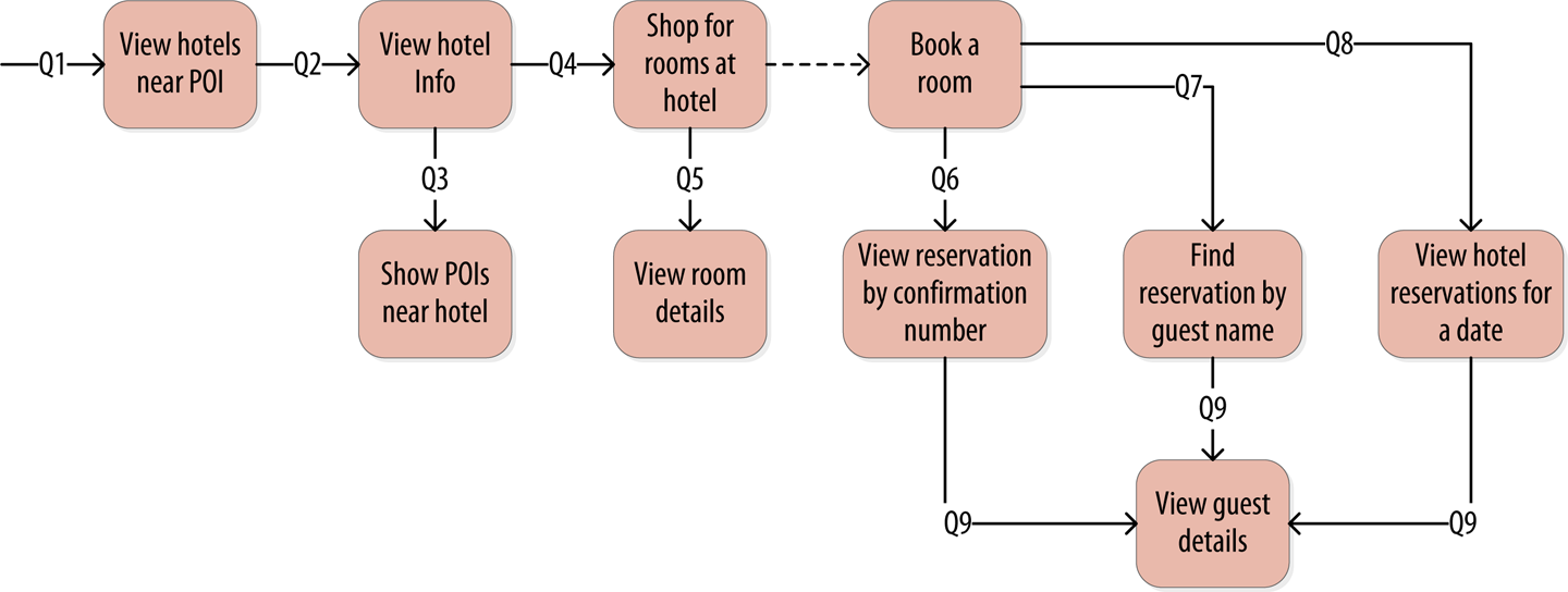
Figure 5-3. Hotel application queries
Logical Data Modeling
Now that you have defined your queries, you’re ready to begin designing Cassandra tables. First, you’ll create a logical model containing a table for each query, capturing entities and relationships from the conceptual model.
To name each table, identify the primary entity type for which you are querying, and use that to start the entity name. If you are querying by attributes of other related entities, you append those to the table name, separated with _by_; for example, hotels_by_poi.
Next, identify the primary key for the table, adding partition key columns based on the required query attributes, and clustering columns in order to guarantee uniqueness and support desired sort ordering.
The Importance of Primary Keys in Cassandra
The design of the primary key is extremely important, as it will determine how much data will be stored in each partition and how that data is organized on disk, which in turn will affect how quickly Cassandra processes read queries.
You complete the design of each table by adding any additional attributes identified by the query. If any of these additional attributes are the same for every instance of the partition key, mark the column as static.
Now that was a pretty quick description of a fairly involved process, so it will be worth your time to work through a detailed example. First, let’s introduce a notation that you can use to represent your logical models.
Hotel Logical Data Model
Figure 5-5 shows a Chebotko logical data model for the queries involving hotels, points of interest, rooms, and amenities. One thing you’ll notice immediately is that the Cassandra design doesn’t include dedicated tables for rooms or amenities, as you had in the relational design. This is because your workflow didn’t identify any queries requiring this direct access.
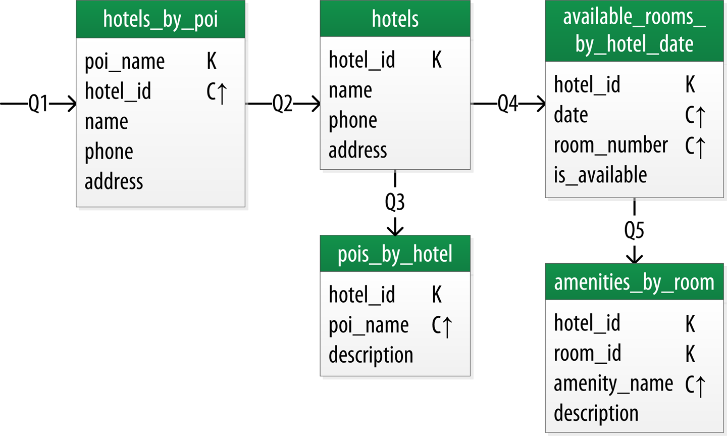
Figure 5-5. Hotel domain logical model
Let’s explore the details of each of these tables.
The first query (Q1) is to find hotels near a point of interest, so you’ll call the table hotels_by_poi. You’re searching by a named point of interest, so that is a clue that the point of interest should be a part of the primary key. Let’s reference the point of interest by name, because according to your workflow that is how your users will start their search.
You’ll note that you certainly could have more than one hotel near a given point of interest, so you’ll need another component in your primary key in order to make sure you have a unique partition for each hotel. So you add the hotel key as a clustering column.
Let’s also assume that according to your application workflow, your user will provide a name of a point of interest, but would benefit from seeing the description of the point of interest alongside hotel results. Therefore you include the poi_description as a column in the hotels_by_poi table, and designate this value as a static column since the point of interest description is the same for all rows in a partition.
Make Your Primary Keys Unique
An important consideration in designing your table’s primary key is making sure that it defines a unique data element. Otherwise you run the risk of accidentally overwriting data.
Now for the second query (Q2), you’ll need a table to get information about a specific hotel. One approach would be to put all of the attributes of a hotel in the hotels_by_poi table, but you choose to add only those attributes required by your application workflow.
From the workflow diagram, you note that the hotels_by_poi table is used to display a list of hotels with basic information on each hotel, and the application knows the unique identifiers of the hotels returned. When the user selects a hotel to view details, you can then use Q2, which is used to obtain details about the hotel. Because you already have the hotel_id from Q1, you use that as a reference to the hotel you’re looking for. Therefore the second table is just called hotels.
Another option would be to store a set of poi_names in the hotels table. This is an equally valid approach. You’ll learn through experience which approach is best for your application.
Q3 is just a reverse of Q1—looking for points of interest near a hotel, rather than hotels near a point of interest. This time, however, you need to access the details of each point of interest, as represented by the pois_by_hotel table. As you did previously, you add the point of interest name as a clustering key to guarantee uniqueness.
At this point, let’s now consider how to support query Q4 to help your users find available rooms at a selected hotel for the nights they are interested in staying. Note that this query involves both a start date and an end date. Because you’re querying over a range instead of a single date, you know that you’ll need to use the date as a clustering key. You use the hotel_id as a primary key to group room data for each hotel on a single partition, which should help your search be super fast. Let’s call this the available_rooms_by_hotel_date table.
Searching Over a Range
Use clustering columns to store attributes that you need to access in a range query. Remember that the order of the clustering columns is important. You’ll learn more about range queries in Chapter 9.
In order to round out the shopping portion of your data model, you add the amenities_by_room table to support Q5. This will allow your user to view the amenities of one of the rooms that is available for the desired stay dates.
Reservation Logical Data Model
Now let’s switch gears to look at the reservation queries. Figure 5-6 shows a logical data model for reservations. You’ll notice that these tables represent a denormalized design; the same data appears in multiple tables, with differing keys.
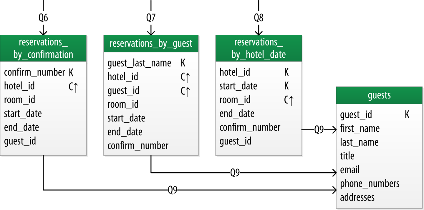
Figure 5-6. A denormalized logical model for reservations
In order to satisfy Q6, the reservations_by_confirmation table supports the lookup of reservations by a unique confirmation number provided to the customer at the time of booking.
If the guest doesn’t have the confirmation number, the reservations_by_guest table can be used to look up the reservation by guest name. You could envision query Q7 being used on behalf of a guest on a self-serve website or a call center agent trying to assist the guest. Because the guest name might not be unique, you include the guest ID here as a clustering column as well.
The hotel staff might wish to see a record of upcoming reservations by date in order to get insight into how the hotel is performing, such as the dates the hotel is sold out or undersold. Q8 supports the retrieval of reservations for a given hotel by date.
Finally, you create a guests table. You’ll notice that it has similar attributes to the user table from Chapter 4. This provides a single location that you can use to store data about guests. In this case, you specify a separate unique identifier for your guest records, as it is not uncommon for guests to have the same name. In many organizations, a customer database such as the guests table would be part of a separate customer management application, which is why we’ve omitted other guest access patterns from this example.
Design Queries for All Stakeholders
Q8 and Q9 in particular help to remind you that you need to create queries that support various stakeholders of your application, not just customers but staff as well, and perhaps even the analytics team, suppliers, and so on.
Physical Data Modeling
Once you have a logical data model defined, creating the physical model is a relatively simple process.
You walk through each of your logical model tables, assigning types to each item. You can use any of the types you learned in Chapter 4, including the basic types, collections, and user-defined types. You may identify additional user-defined types that can be created to simplify your design.
After you’ve assigned data types, you analyze your model by performing size calculations and testing out how the model works. You may make some adjustments based on your findings. Once again, let’s cover the data modeling process in more detail by working through an example.
First, let’s look at a few additions to the Chebotko notation for physical data models.
Hotel Physical Data Model
Now let’s get to work on your physical model. First, you need keyspaces to contain your tables. To keep the design relatively simple, you create a hotel keyspace to contain tables for hotel and availability data, and a reservation keyspace to contain tables for reservation and guest data. In a real system, you might divide the tables across even more keyspaces in order to separate concerns.
For the hotels table, you use Cassandra’s text type to represent the hotel’s id. For the address, you use the address type similar to the one you created in Chapter 4. You use the text type to represent the phone number, as there is considerable variance in the formatting of numbers between countries.
Using Unique Identifiers as References
While it would make sense to use the uuid type for attributes such as the hotel_id, for the purposes of this book we mostly use text attributes as identifiers, to keep the samples simple and readable. For example, a common convention in the hospitality industry is to reference properties by short codes like “AZ123” or “NY229.” We’ll use these values for hotel_ids, while acknowledging they are not necessarily globally unique.
You’ll find that it’s often helpful to use unique IDs to uniquely reference elements, and to use these uuids as references in tables representing other entities. This helps to minimize coupling between different entity types. This may prove especially effective if you are using a microservice architectural style for your application, in which there are separate services responsible for each entity type.
As you work to create physical representations of various tables in your logical hotel data model, you use the same approach. The resulting design is shown in Figure 5-8.
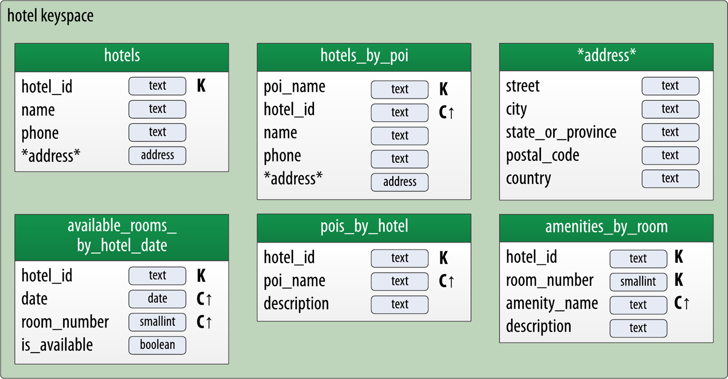
Figure 5-8. Hotel physical model
The address type is also included in the design, designated with an asterisk to denote that it is a user-defined type, and has no primary key columns identified. You make use of this type in the hotels and hotels_by_poi tables.
Taking Advantage of User-Defined Types
User-defined types are frequently used to create logical groupings of nonprimary key columns, as you have done with the address user-defined type. UDTs can also be stored in collections to further reduce complexity in the design.
Remember that the scope of a UDT is the keyspace in which it is defined. To use address in the reservation keyspace you’re about to design, you’ll have to declare it again.
Reservation Physical Data Model
Now, let’s examine the reservation tables in your design. Remember that your logical model contained three denormalized tables to support queries for reservations by confirmation number, guest, and hotel and date. For the first iteration of your physical data model design, let’s assume you’re going to manage this denormalization manually (see Figure 5-9). (We’ll revisit this design choice in Chapter 7 to consider using Cassandra’s materialized view feature.)
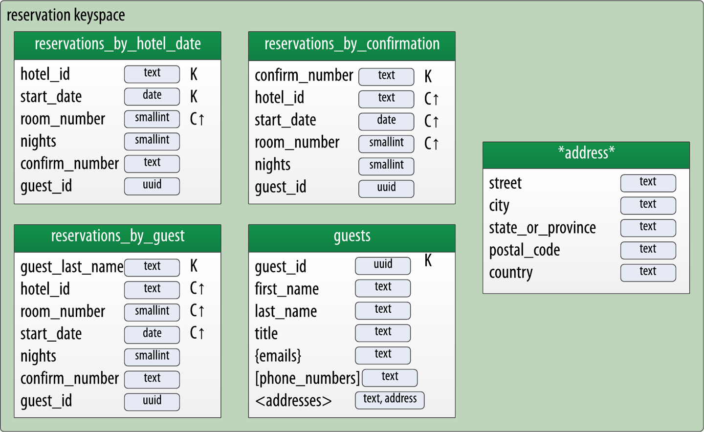
Figure 5-9. Reservation physical model
Note that you have reproduced the address type in this keyspace and modeled the guest_id as a uuid type in all of your tables.
Evaluating and Refining
Once you’ve created your physical model, there are some steps you’ll want to take to evaluate and refine your table designs to help ensure optimal performance.
Calculating Partition Size
The first thing that you want to look for is whether your tables will have partitions that will be overly large, or to put it another way, too wide. Partition size is measured by the number of cells (values) that are stored in the partition. Cassandra’s hard limit is two billion cells per partition, but you’ll likely run into performance issues before reaching that limit. The recommended size of a partition is not more than 100,000 cells.
In order to calculate the size of your partitions, you use the following formula:
The number of values (or cells) in the partition (Nv) is equal to the number of static columns (Ns) plus the product of the number of rows (Nr) and the number of of values per row. The number of values per row is defined as the number of columns (Nc) minus the number of primary key columns (Npk) and static columns (Ns).
The number of columns tends to be relatively static, although as you have seen, it is quite possible to alter tables at runtime. For this reason, a primary driver of partition size is the number of rows in the partition. This is a key factor that you must consider in determining whether a partition has the potential to get too large. Two billion values sounds like a lot, but in a sensor system where tens or hundreds of values are measured every millisecond, the number of values starts to add up pretty fast.
Let’s take a look at one of your tables to analyze the partition size. Because it has a wide partition design with one partition per hotel, you choose the available_rooms_by_hotel_date table. The table has four columns total (Nc = 4), including three primary key columns (Npk = 3) and no static columns (Ns = 0). Plugging these values into the formula, you get:
Therefore the number of values for this table is equal to the number of rows. You still need to determine a number of rows. To do this, you make some estimates based on the application you’re designing. The table is storing a record for each room, in each of your hotels, for every night. Let’s assume that your system will be used to store 2 years of inventory at a time, and there are 5,000 hotels in the system, with an average of 100 rooms in each hotel.
Since there is a partition for each hotel, the estimated number of rows per partition is as follows:
This relatively small number of rows per partition is not an issue, but the number of cells may be. If you start storing more dates of inventory, or don’t manage the size of your inventory well using TTL, you could start having issues. You still might want to look at breaking up this large partition, which you’ll learn how to do shortly.
Calculating Size on Disk
In addition to calculating the size of your partitions, it is also an excellent idea to estimate the amount of disk space that will be required for each table you plan to store in the cluster. In order to determine the size, you use the following formula to determine the size St of a partition:
This is a bit more complex than the previous formula, but let’s break it down a bit at a time, starting with the notation:
-
In this formula, ck refers to partition key columns, cs to static columns, cr to regular columns, and cc to clustering columns.
-
The termavg refers to the average number of bytes of metadata stored per cell, such as timestamps. It is typical to use an estimate of 8 bytes for this value.
-
You recognize the number of rows Nr and number of values Nv from previous calculations.
-
The sizeOf() function refers to the size, in bytes, of the CQL data type of each referenced column.
The first term asks you to sum the size of the partition key columns. For this design, the available_rooms_by_hotel_date table has a single partition key column, the hotel_id, which you chose to make of type text. Assuming your hotel identifiers are simple 5-character codes, you have a 5-byte value, so the sum of the partition key column sizes is 5 bytes.
The second term asks you to sum the size of your static columns. This table has no static columns, so in your case this is 0 bytes.
The third term is the most involved, and for good reason—it is calculating the size of the cells in the partition. You sum the size of the clustering columns and regular columns. The clustering columns are the date, which is 4 bytes, and the room_number, which is a 2-byte short integer, giving a sum of 6 bytes. There is only a single regular column, the boolean is_available, which is 1 byte in size. Summing the regular column size (1 byte) plus the clustering column size (6 bytes) gives a total of 7 bytes. To finish up the term, you multiply this value by the number of rows (73,000), giving a result of 511,000 bytes (0.51 MB).
The fourth term is simply counting the metadata that Cassandra stores for each cell. In the storage format used by Cassandra 3.0 and later, the amount of metadata for a given cell varies based on the type of data being stored, and whether or not custom timestamp or TTL values are specified for individual cells. For your table, you reuse the number of values from the previous calculation (73,000) and multiply by 8, which gives a result of 0.58 MB.
Adding these terms together, you get the final estimate:
Partition size = 16 bytes + 0 bytes + 0.51 MB + 0.58 MB = 1.1 MB
This formula is an approximation of the uncompressed size of a partition on disk, but is accurate enough to be quite useful. (Note that if you make use of SSTable compression, as discussed in Chapter 13, the storage space required will be reduced.) Remembering that the partition must be able to fit on a single node, it looks like your table design will not put a lot of strain on your disk storage.
A More Compact Storage Format
As mentioned in Chapter 2, Cassandra’s storage engine was re-implemented for the 3.0 release, including a new format for SSTable files. The previous format stored a separate copy of the clustering columns as part of the record for each cell. The newer format eliminates this duplication, which reduces the size of stored data and simplifies the formula for computing that size.
Keep in mind also that this estimate only counts a single replica of your data. You will need to multiply the value obtained here by the number of partitions and the number of replicas specified by the keyspace’s replication strategy in order to determine the total required capacity for each table. This will come in handy when you learn how to plan cluster deployments in Chapter 10.
Breaking Up Large Partitions
As discussed previously, your goal is to design tables that can provide the data you need with queries that touch a single partition, or failing that, the minimum possible number of partitions. However, as you have seen in previous examples, it is quite possible to design wide partition–style tables that approach Cassandra’s built-in limits. Performing sizing analysis on tables may reveal partitions that are potentially too large, either in number of values, size on disk, or both.
The technique for splitting a large partition is straightforward: add an additional column to the partition key. In most cases, moving one of the existing columns into the partition key will be sufficient. Another option is to introduce an additional column to the table to act as a sharding key, but this requires additional application logic.
Continuing to examine the available rooms example, if you add the date column to the partition key for the available_rooms_by_hotel_date table, each partition would then represent the availability of rooms at a specific hotel on a specific date. This will certainly yield partitions that are significantly smaller, perhaps too small, as the data for consecutive days will likely be on separate nodes. This also increases your effort to do queries that span multiple days, as you will have to query multiple partitions.
Another technique, known as bucketing, is often used to break the data into moderate-size partitions. For example, you could bucketize the available_rooms_by_hotel_date table by adding a month column to the partition key, perhaps represented as an integer. The comparision with the original design is shown in Figure 5-10. While the month column is partially duplicative of the date, it provides a nice way of grouping related data in a partition that will not get too large.
If you really felt strongly about preserving a wide partition design, you could instead add the room_id to the partition key, so that each partition would represent the availability of the room across all dates. Because you haven’t identified a query that involves searching availability of a specific room, the first or second design approach is most suitable to your application needs.
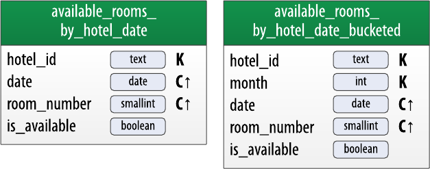
Figure 5-10. Adding a month bucket to the available_rooms_by_hotel_date table
Defining Database Schema
Once you have finished evaluating and refining your physical model, you’re ready to implement the schema in CQL. Here is the schema for the hotel keyspace, using CQL’s comment feature to document the query pattern supported by each table:
CREATE KEYSPACE hotel
    WITH replication = {'class': 'SimpleStrategy', 'replication_factor' : 3};

CREATE TYPE hotel.address (
    street text,
    city text,
    state_or_province text,
    postal_code text,
    country text
);

CREATE TABLE hotel.hotels_by_poi (
    poi_name text,
    poi_description text STATIC,
    hotel_id text,
    name text,
    phone text,
    address frozen<address>,
    PRIMARY KEY ((poi_name), hotel_id)
) WITH comment = 'Q1. Find hotels near given poi'
AND CLUSTERING ORDER BY (hotel_id ASC) ;

CREATE TABLE hotel.hotels (
    id text PRIMARY KEY,
    name text,
    phone text,
    address frozen<address>,
    pois set<text>
) WITH comment = 'Q2. Find information about a hotel';

CREATE TABLE hotel.pois_by_hotel (
    poi_name text,
    hotel_id text,
    description text,
    PRIMARY KEY ((hotel_id), poi_name)
) WITH comment = 'Q3. Find pois near a hotel';

CREATE TABLE hotel.available_rooms_by_hotel_date (
    hotel_id text,
    date date,
    room_number smallint,
    is_available boolean,
    PRIMARY KEY ((hotel_id), date, room_number)
) WITH comment = 'Q4. Find available rooms by hotel / date';

CREATE TABLE hotel.amenities_by_room (
    hotel_id text,
    room_number smallint,
    amenity_name text,
    description text,
    PRIMARY KEY ((hotel_id, room_number), amenity_name)
) WITH comment = 'Q5. Find amenities for a room';
Identify Partition Keys Explicitly
We recommend representing tables by surrounding the elements of your partition key with parentheses, even though the partition key consists of the single column poi_name. This is a best practice that makes your selection of partition key more explicit to others reading your CQL.
Similarly, here is the schema for the reservation keyspace:
CREATE KEYSPACE reservation
    WITH replication = {'class': 'SimpleStrategy', 'replication_factor' : 3};

CREATE TYPE reservation.address (
    street text, city text,
    state_or_province text,
    postal_code text,
    country text
);

CREATE TABLE reservation.reservations_by_confirmation (
    confirm_number text,
    hotel_id text,
    start_date date,
    end_date date,
    room_number smallint,
    guest_id uuid,
    PRIMARY KEY (confirm_number)
) WITH comment = 'Q6. Find reservations by confirmation number';

CREATE TABLE reservation.reservations_by_hotel_date (
    hotel_id text,
    start_date date,
    end_date date,
    room_number smallint,
    confirm_number text,
    guest_id uuid,
    PRIMARY KEY ((hotel_id, start_date), room_number)
) WITH comment = 'Q7. Find reservations by hotel and date';

CREATE TABLE reservation.reservations_by_guest (
    guest_last_name text,
    hotel_id text,
    start_date date,
    end_date date,
    room_number smallint,
    confirm_number text,
    guest_id uuid,
    PRIMARY KEY ((guest_last_name), hotel_id)
) WITH comment = 'Q8. Find reservations by guest name';

CREATE TABLE reservation.guests (
    guest_id uuid PRIMARY KEY,
    first_name text,
    last_name text,
    title text,
    emails set<text>,
    phone_numbers list<text>,
    addresses map<text, frozen<address>>,
    confirm_number text
) WITH comment = 'Q9. Find guest by ID';
You now have a complete Cassandra schema for storing data for your hotel application.
Cassandra Data Modeling Tools
You’ve already had quite a bit of practice creating schema and manipluating data using cqlsh, but now that you’re starting to create an application data model with more tables, it starts to be more of a challenge to keep track of all of that CQL.
Thankfully, there are several tools available to help you design and manage your Cassandra schema and build queries:
- Hackolade
-
Hackolade is a data modeling tool that supports schema design for Cassandra and many other NoSQL databases. Hackolade supports the unique concepts of CQL, such as partition keys and clustering columns, as well as data types, including collections and UDTs. It also provides the ability to create Chebotko diagrams, as described in this chapter. Figure 5-11 shows an entity-relationship diagram representing the conceptual data model from this chapter.
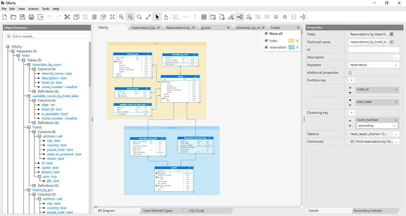
Figure 5-11. An entity-relationship diagram for hotel and reservation data in Hackolade
- Kashlev Data Modeler
-
The Kashlev Data Modeler is a Cassandra data modeling tool that automates the data modeling methodology described in this chapter, including identifying access patterns; conceptual, logical, and physical data modeling; and schema generation. It also includes model patterns that you can optionally leverage as a starting point for your designs.
- DataStax DevCenter
-
DataStax DevCenter is a tool for managing schema, executing queries, and viewing results. While the tool is no longer actively supported, it is still popular with many developers and is available as a free download from DataStax. Figure 5-12 shows the hotel schema being edited in DevCenter.
The middle pane shows the currently selected CQL file, featuring syntax highlighting for CQL commands, CQL types, and name literals. DevCenter provides command completion as you type out CQL commands, and interprets the commands you type, highlighting any errors you make. The tool provides panes for managing multiple CQL scripts and connections to multiple clusters. The connections are used to run CQL commands against live clusters and view the results. The tool also has a query trace feature that is useful for gaining insight into the performance of your queries.
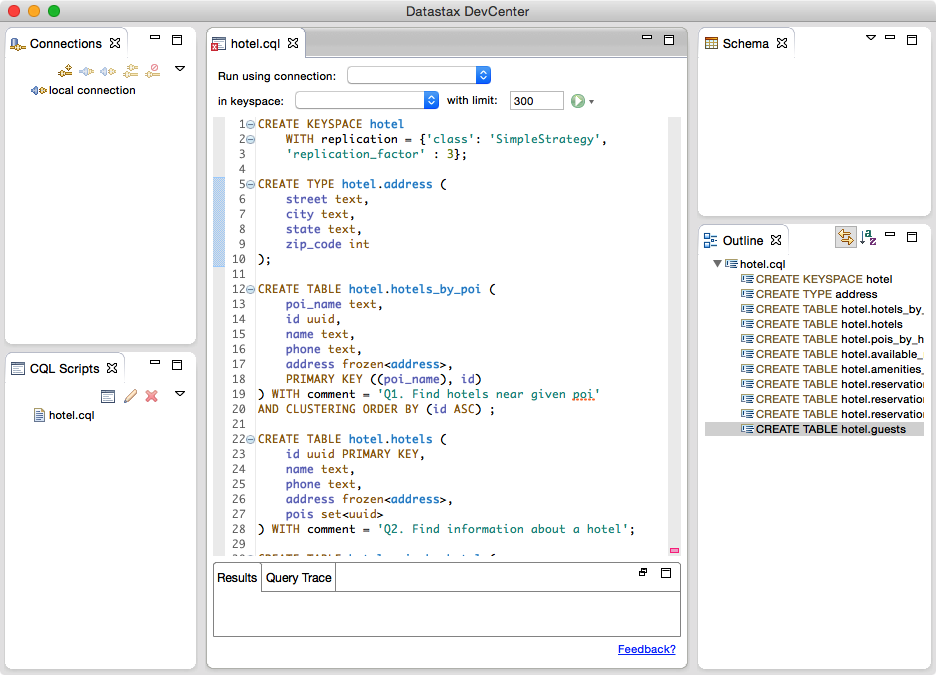
Figure 5-12. Editing the hotel schema in DataStax DevCenter
- IDE plug-ins
-
CQL plug-ins are available for several integrated development environments (IDEs), such as IntelliJ IDEA and Apache NetBeans. These plug-ins typically provide features such as schema management and query execution.
Make Sure Your Tools Have Full CQL Support
Some IDEs and tools that claim to support Cassandra do not actually support CQL natively, but instead access Cassandra using a JDBC/ODBC driver and interact with Cassandra as if it were a relational database with SQL support. When selecting tools for working with Cassandra, you’ll want to make sure they support CQL and reinforce Cassandra best practices for data modeling, as discussed in this chapter.
Summary
In this chapter, you learned how to create a complete, working Cassandra data model and compared it with an equivalent relational model. You represented the data model in both logical and physical forms, and learned about tools for realizing your data models in CQL. Now that you have a working data model, you’re ready to continue building a hotel application in the coming chapters.