Chapter 3

The Components of SQL

IN THIS CHAPTER

Creating databases

Manipulating data

Protecting databases

SQL is a special-purpose language designed for the creation and maintenance of data in relational databases. Although the vendors of relational database management systems have their own SQL implementations, an ISO/IEC standard (revised in 2016) defines and controls what SQL is. All implementations differ from the standard to varying degrees. Close adherence to the standard is the key to running a database (and its associated applications) on more than one platform.

Although SQL isn’t a general-purpose programming language, it contains some impressive tools. Three languages within the language offer everything you need to create, modify, maintain, and provide security for a relational database:

• The Data Definition Language (DDL): The part of SQL that you use to create (completely define) a database, modify its structure, and destroy it when you no longer need it.
• The Data Manipulation Language (DML): The part of SQL that performs database maintenance. Using this powerful tool, you can specify what you want to do with the data in your database — enter it, change it, remove it, or retrieve it.
• The Data Control Language (DCL): The part of SQL that protects your database from becoming corrupted. Used correctly, the DCL provides security for your database; the amount of protection depends on the implementation. If your implementation doesn’t provide sufficient protection, you must add that protection to your application program.

This chapter introduces the DDL, DML, and DCL.

Data Definition Language

The Data Definition Language (DDL) is the part of SQL you use to create, change, or destroy the basic elements of a relational database. Basic elements include tables, views, schemas, catalogs, clusters, and possibly other things as well. In the following sections, I discuss the containment hierarchy that relates these elements to each other and look at the commands that operate on these elements.

In Chapter 1, I mention tables and schemas, noting that a schema is an overall structure that includes tables within it. Tables and schemas are two elements of a relational database’s containment hierarchy. You can break down the containment hierarchy as follows:

• Tables contain columns and rows.
• Schemas contain tables and views.
• Catalogs contain schemas.

The database itself contains catalogs. Sometimes the database is referred to as a cluster. I mention clusters again later in this chapter, in the section on ordering by catalog.

When “Just do it!” is not good advice

Suppose you set out to create a database for your organization. Excited by the prospect of building a useful, valuable, and totally righteous structure of great importance to your company’s future, you sit down at your computer and start entering SQL CREATE statements. Right?

Well, no. Not quite. In fact, that's a prescription for disaster. Many database-development projects go awry from the start as excitement and enthusiasm overtake careful planning. Even if you have a clear idea of how to structure your database, write everything down on paper before touching your keyboard.

Here’s where database development bears some resemblance to a game of chess. In the middle of a complicated and competitive chess game, you may see what looks like a good move. The urge to make that move can be overwhelming. However, the odds are good that you’ve missed something. Grandmasters advise newer players — only partly in jest — to sit on their hands. If sitting on your hands prevents you from making an ill-advised move, then so be it: Sit on your hands. If you study the position a little longer, you might find an even better move — or you might even see a brilliant counter move that your opponent can make. Plunging into creating a database without sufficient forethought can lead to a database structure that, at best, is suboptimal. At worst, it could be disastrous, an open invitation to data corruption. Sitting on your hands probably won’t help, but it will help to pick up a pencil in one of those hands and start mapping your database plan on paper. For help in deciding what to include in your plan, check out my book Database Development For Dummies, which covers planning in depth.

Keep in mind the following procedures when planning your database:

• Identify all tables.
• Define the columns that each table must contain.
• Give each table a primary key that you can guarantee is unique. (I discuss primary keys in Chapters 4 and 5.)
• Make sure that every table in the database has at least one column in common with (at least) one other table in the database. These shared columns serve as logical links that enable you to relate information in one table to the corresponding information in another table.
• Put each table in third normal form (3NF) or better, to ensure the prevention of insertion, deletion, and update anomalies. (I discuss database normalization in Chapter 5.)

After you complete the design on paper and verify that it’s sound, you’re ready to transfer the design to the computer. You can do this bit of magic by typing SQL CREATE statements. More likely, you will use your DBMS’s graphical user interface (GUI) to create the elements of your design. If you do use a GUI, your input will be converted “under the covers” into SQL by your DBMS.

Creating tables

A database table looks a lot like a spreadsheet table: a two-dimensional array made up of rows and columns. You can create a table by using the SQL CREATE TABLE command. Within the command, you specify the name and data type of each column.

After you create a table, you can start loading it with data. (Loading data is a DML, not a DDL, function.) If requirements change, you can change a table's structure by using the ALTER TABLE command. If a table outlives its usefulness or becomes obsolete, you can eliminate it with the DROP command. The various forms of the CREATE and ALTER commands, together with the DROP command, make up SQL's DDL.

Suppose you’re a database designer and you don’t want your database tables to turn to guacamole as you make updates over time. You decide to structure your database tables according to the best normalized form so that you can maintain data integrity.

Normalization, an extensive field of study in its own right, is a way of structuring database tables so that updates don’t introduce anomalies. Each table you create contains columns that correspond to attributes that are tightly linked to each other.

You may, for example, create a CUSTOMER table with the attributes CUSTOMER.CustomerID, CUSTOMER.FirstName, CUSTOMER.LastName, CUSTOMER.Street, CUSTOMER.City, CUSTOMER.State, CUSTOMER.Zipcode, and CUSTOMER.Phone. All these attributes are more closely related to the customer entity than to any other entity in a database that may contain many tables. These attributes contain all the relatively permanent customer information that your organization keeps on file.

Most database management systems provide a graphical tool for creating database tables. You can also create such tables by using an SQL command. The following example demonstrates a command that creates your CUSTOMER table:

CREATE TABLE CUSTOMER (

CustomerID INTEGER NOT NULL,

FirstName CHAR (15),

LastName CHAR (20) NOT NULL,

Street CHAR (25),

City CHAR (20),

State CHAR (2),

Zipcode CHAR (10),

Phone CHAR (13) ) ;

For each column, you specify its name (for example, CustomerID), its data type (for example, INTEGER), and possibly one or more constraints (for example, NOT NULL).

Figure 3-1 shows a portion of the CUSTOMER table with some sample data.

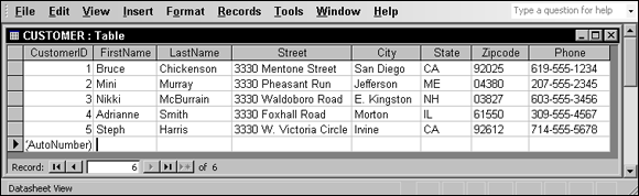
FIGURE 3-1: Use the CREATE TABLE command to create this CUSTOMER table.

If the SQL implementation you use doesn't fully implement the latest version of ISO/IEC standard SQL, the syntax you need to use may differ from the syntax that I give in this book. Read the user documentation that came with your DBMS for specific information.

A room with a view

At times, you want to retrieve specific information from the CUSTOMER table. You don’t want to look at everything — only specific columns and rows. What you need is a view.

A view is a virtual table. In most implementations, a view has no independent physical existence. The view’s definition exists only in the database’s metadata, but the data comes from the table or tables from which you derive the view. The view’s data is not physically duplicated somewhere else in online disk storage. Some views consist of specific columns and rows of a single table. Others, known as multi-table views, draw from two or more tables.

Single-table view

Sometimes when you have a question, the data that gives you the answer resides in a single table in your database. If the information you want exists in a single table, you can create a single-table view of the data. For example, suppose you want to look at the names and telephone numbers of all customers who live in the state of New Hampshire. You can create a view from the CUSTOMER table that contains only the data you want. The following SQL statement creates this view:

CREATE VIEW NH_CUST AS

SELECT CUSTOMER.FirstName,

CUSTOMER.LastName,

CUSTOMER.Phone

FROM CUSTOMER

WHERE CUSTOMER.State = 'NH' ;

Figure 3-2 shows how you derive the view from the CUSTOMER table.

FIGURE 3-2: You derive the NH_CUST view from the CUSTOMER table.

This code is correct, but a little on the wordy side. You can accomplish the same task with less typing if your SQL implementation assumes that all table references are the same as the ones in the FROM clause. If your system makes that reasonable default assumption, you can reduce the statement to the following lines:

CREATE VIEW NH_CUST AS

SELECT FirstName, LastName, Phone

FROM CUSTOMER

WHERE STATE = 'NH';

Although the second version is easier to write and read, it’s more vulnerable to disruption from ALTER TABLE commands. Such disruption isn't a problem for this simple case, which has no JOIN, but views with JOINs are more robust when they use fully qualified names. I cover JOINs in Chapter 11.

Creating a multi-table view

Quite often, you need to pull data from two or more tables to answer your question. Suppose, for example, that you work for a sporting goods store, and you want to send a promotional mailing to all the customers who have bought ski equipment since the store opened last year. You need information from the CUSTOMER table, the PRODUCT table, the INVOICE table, and the INVOICE_LINE table. You can create a multi-table view that shows the data you need. After you create the view, you can use that same view again and again. Each time you use the view, it reflects any changes that occurred in the underlying tables since you last used the view.

The database for this sporting goods store contains four tables: CUSTOMER, PRODUCT, INVOICE, and INVOICE_LINE. The tables are structured as shown in Table 3-1.

TABLE 3-1 Sporting Goods Store Database Tables

Table	Column	Data Type	Constraint
CUSTOMER	CustomerID	INTEGER	NOT NULL
	FirstName	CHAR (15)
	LastName	CHAR (20)	NOT NULL
	Street	CHAR (25)
	City	CHAR (20)
	State	CHAR (2)
	Zipcode	CHAR (10)
	Phone	CHAR (13)
PRODUCT	ProductID	INTEGER	NOT NULL
	Name	CHAR (25)
	Description	CHAR (30)
	Category	CHAR (15)
	VendorID	INTEGER
	VendorName	CHAR (30)
INVOICE	InvoiceNumber	INTEGER	NOT NULL
	CustomerID	INTEGER
	InvoiceDate	DATE
	TotalSale	NUMERIC (9,2)
	TotalRemitted	NUMERIC (9,2)
	FormOfPayment	CHAR (10)
INVOICE_LINE	LineNumber	INTEGER	NOT NULL
	InvoiceNumber	INTEGER	NOT NULL
	ProductID	INTEGER	NOT NULL
	Quantity	INTEGER
	SalePrice	NUMERIC (9,2)

Notice that some of the columns in Table 3-1 contain the constraint NOT NULL. These columns are either the primary keys of their respective tables or columns that you decide must contain a value. A table's primary key must uniquely identify each row. To do that, the primary key must contain a non-null value in every row. (I discuss keys in detail in Chapter 5.)

The tables relate to each other through the columns that they have in common. The following list describes these relationships (as shown in Figure 3-3):

• The CUSTOMER table bears a one-to-many relationship to the INVOICE table. One customer can make multiple purchases, generating multiple invoices. Each invoice, however, deals with one, and only one, customer.
• The INVOICE table bears a one-to-many relationship to the INVOICE_LINE table. An invoice may have multiple lines, but each line appears on one, and only one, invoice.
• The PRODUCT table also bears a one-to-many relationship to the INVOICE_LINE table. A product may appear on more than one line on one or more invoices. Each line, however, deals with one, and only one, product.

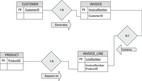
FIGURE 3-3: A sporting goods store’s database structure.

The CUSTOMER table links to the INVOICE table by the common CustomerID column. The INVOICE table links to the INVOICE_LINE table by the common InvoiceNumber column. The PRODUCT table links to the INVOICE_LINE table by the common ProductID column. These links are what make this database a relational database.

To access the information about customers who bought ski equipment, you need FirstName, LastName, Street, City, State, and Zipcode from the CUSTOMER table; Category from the PRODUCT table; InvoiceNumber from the INVOICE table; and LineNumber from the INVOICE_LINE table. You can create the view you want in stages by using the following statements:

CREATE VIEW SKI_CUST1 AS

SELECT FirstName,

LastName,

Street,

City,

State,

Zipcode,

InvoiceNumber

FROM CUSTOMER JOIN INVOICE

USING (CustomerID) ;

CREATE VIEW SKI_CUST2 AS

SELECT FirstName,

LastName,

Street,

City,

State,

Zipcode,

ProductID

FROM SKI_CUST1 JOIN INVOICE_LINE

USING (InvoiceNumber) ;

CREATE VIEW SKI_CUST3 AS

SELECT FirstName,

LastName,

Street,

City,

State,

Zipcode,

Category

FROM SKI_CUST2 JOIN PRODUCT

USING (ProductID) ;

CREATE VIEW SKI_CUST AS

SELECT DISTINCT FirstName,

LastName,

Street,

City,

State,

Zipcode

FROM SKI_CUST3

WHERE CATEGORY = 'Ski' ;

These CREATE VIEW statements combine data from multiple tables by using the JOIN operator. Figure 3-4 diagrams the process.

FIGURE 3-4: Creating a multi-table view by using JOINs.

Here's a rundown of the four CREATE VIEW statements:

• The first statement combines columns from the CUSTOMER table with a column of the INVOICE table to create the SKI_CUST1 view.
• The second statement combines SKI_CUST1 with a column from the INVOICE_LINE table to create the SKI_CUST2 view.
• The third statement combines SKI_CUST2 with a column from the PRODUCT table to create the SKI_CUST3 view.

• The fourth statement filters out all rows that don't have a category of Ski. The result is a view (SKI_CUST) that contains the names and addresses of all customers who bought at least one product in the Ski category.

  The DISTINCT keyword in the fourth CREATE VIEW's SELECT clause ensures that you have only one entry for each customer, even if some customers made multiple purchases of ski items. (I cover JOINs in detail in Chapter 11.)

It's possible to create a multi-table view with a single SQL statement. However, if you think that one or all of the preceding statements are complex, imagine how complex a single statement would be that performed all these functions. I tend to prefer simplicity over complexity, so whenever possible, I choose the simplest way to perform a function, even if it is not the most “efficient.”

Collecting tables into schemas

A table consists of rows and columns and usually deals with a specific type of entity, such as customers, products, or invoices. Useful work generally requires information about several (or many) related entities. Organizationally, you collect the tables that you associate with these entities according to a logical schema. A logical schema is the organizational structure of a collection of related tables.

A database also has a physical schema — which represents the physical arrangement of the data and its associated items (such as indexes) on the system’s storage devices. When I mention “the schema” of a database, I’m referring to the logical schema, not the physical schema.

On a system where several unrelated projects may co-reside, you can assign all related tables to one schema. You can collect other groups of tables into schemas of their own.

Be sure to name your schemas to ensure that no one accidentally mixes tables from one project with tables from another. Each project has its own associated schema; you can distinguish it from other schemas by name. Seeing certain table names (such as CUSTOMER, PRODUCT, and so on) appear in multiple projects, however, is common. If any chance exists of a naming ambiguity, qualify your table name by using its schema name as well (as in SCHEMA_NAME.TABLE_NAME). If you don’t qualify a table name, SQL assigns that table to the default schema.

Ordering by catalog

For really large database systems, multiple schemas may not be sufficient. In a large distributed database environment with many users, you may even find duplicated schema names. To prevent this situation, SQL adds another level to the containment hierarchy: the catalog. A catalog is a named collection of schemas.

You can qualify a table name by using a catalog name and a schema name. This safeguard is the best way to ensure that no one confuses the table in one schema with a table that has the same name in some other schema that has the same schema name. (Say what? Well, some folks just have a really hard time thinking up different names.) The catalog-qualified name appears in the following format:

CATALOG_NAME.SCHEMA_NAME.TABLE_NAME

At the top of the database containment hierarchy are clusters. Systems rarely require use of the full scope of the containment hierarchy; going to the catalog level is enough in most cases. A catalog contains schemas; a schema contains tables and views; tables and views contain columns and rows.

The catalog also contains the information schema. The information schema contains the system tables. The system tables hold the metadata associated with the other schemas. In Chapter 1, I define a database as a self-describing collection of integrated records. The metadata contained in the system tables is what makes the database self-describing.

Because catalogs are identified by name, you can have multiple catalogs in a database. Each catalog can have multiple schemas, and each schema can have multiple tables. Of course, each table can have multiple columns and rows. The hierarchical relationships are shown in Figure 3-5.

FIGURE 3-5: The hierarchical structure of a typical SQL database.

Getting familiar with DDL statements

SQL’s Data Definition Language (DDL) deals with the structure of a database. It’s distinct from the Data Manipulation Language (described later in this chapter), which deals with the data contained within that structure. The DDL consists of these three statements:

• CREATE: You use the various forms of this statement to build the essential structures of the database.
• ALTER: You use this statement to change structures that you have created.
• DROP: You apply this statement to structures created with the CREATE statement, to destroy them.

In the following sections, I give you brief descriptions of the DDL statements. In Chapters 4 and 5, I use these statements in examples.

CREATE

You can apply the SQL CREATE statement to a large number of SQL objects, including schemas, domains, tables, and views. By using the CREATE SCHEMA statement, you can not only create a schema, but also identify its owner and specify a default character set. Here's an example of such a statement:

CREATE SCHEMA SALES

AUTHORIZATION SALES_MGR

DEFAULT CHARACTER SET ASCII_FULL ;

Use the CREATE DOMAIN statement to apply constraints to column values. The constraints you apply to a domain determine what objects the domain can and cannot contain. You can create domains after you establish a schema. The following example shows how to use this statement:

CREATE DOMAIN Age AS INTEGER

CHECK (AGE > 20) ;

You create tables by using the CREATE TABLE statement, and you create views by using the CREATE VIEW statement. Earlier in this chapter, I show you examples of these two statements. When you use the CREATE TABLE statement, you can specify constraints on the new table's columns at the same time.

Sometimes you may want to specify constraints that don’t specifically attach to a table but apply to an entire schema. You can use the CREATE ASSERTION statement to specify such constraints.

You also have CREATE CHARACTER SET, CREATE COLLATION, and CREATE TRANSLATION statements, which give you the flexibility of creating new character sets, collation sequences, or translation tables. (Collation sequences define the order in which you carry out comparisons or sorts. Translation tables control the conversion of character strings from one character set to another.) You can create a number of other things (which I won't go into here), as you can deduce if you flip to Chapter 2 for a glance at Table 2-1.

ALTER

After you create a table, you’re not necessarily stuck with that exact table forever. As you use the table, you may discover that it’s not everything you need it to be. You can use the ALTER TABLE statement to change the table by adding, changing, or deleting a column in the table. Besides tables, you can also ALTER columns and domains.

DROP

Removing a table from a database schema is easy. Just use a DROP TABLE<tablename> statement. You erase all data from the table, as well as the metadata that defines the table in the data dictionary. It's almost as if the table never existed. You can also use the DROP statement to get rid of anything that was created by a CREATE statement.

DROP won't work if it breaks referential integrity. I discuss referential integrity later in this chapter.

Data Manipulation Language

Although the DDL is the part of SQL that creates, modifies, or destroys database structures, it doesn’t deal with data itself. Handling data is the job of the Data Manipulation Language (DML). Some DML statements read like ordinary English-language sentences and are easy to understand. Unfortunately, because SQL gives you very fine-grained control of your data, other DML statements can be fiendishly complex.

If a DML statement includes multiple expressions, clauses, predicates (more about them later in this chapter), or subqueries, understanding what that statement is trying to do can be a challenge. After you deal with some of these statements, you may even consider switching to an easier line of work, such as brain surgery or quantum electrodynamics. Fortunately, such drastic action isn’t necessary. You can understand complex SQL statements by breaking them down into their basic components and analyzing them one chunk at a time.

The DML statements you can use are INSERT, UPDATE, DELETE, MERGE, and SELECT. These statements can consist of a variety of parts, including multiple clauses. Each clause may incorporate value expressions, logical connectives, predicates, aggregate functions, and subqueries. You can make fine discriminations among database records and extract more information from your data by including these clauses in your statements. In Chapter 6, I discuss the operation of the DML commands, and in Chapters 7 through 13, I delve into the details of these commands.

Value expressions

You can use value expressions to combine two or more values. Several kinds of value expressions exist, corresponding to the different data types:

• Numeric
• String
• Datetime
• Interval
• Boolean
• User-defined
• Row
• Collection

The Boolean, user-defined, row, and collection types were introduced with SQL:1999. Some implementations may not support them all yet. If you want to use these data types, make sure your implementation includes the ones you want to use.

Numeric value expressions

To combine numeric values, use the addition (+), subtraction (-), multiplication (*), and division (/) operators. The following lines are examples of numeric value expressions:

12 – 7

15/3 - 4

6 * (8 + 2)

The values in these examples are numeric literals. These values may also be column names, parameters, host variables, or subqueries — provided that those column names, parameters, host variables, or subqueries evaluate to a numeric value. The following are some examples:

SUBTOTAL + TAX + SHIPPING

6 * MILES/HOURS

:months/12

The colon in the last example signals that the following term (months) is either a parameter or a host variable.

String value expressions

String value expressions may include the concatenation operator (||). Use concatenation to join two text strings, as shown in Table 3-2.

TABLE 3-2 Examples of String Concatenation

Expression	Result
'military ' || 'intelligence'	'military intelligence'
CITY|| ' ' ||STATE|| ' '||ZIP	A single string with city, state, and zip code, each separated by a single space.

Some SQL implementations use + as the concatenation operator rather than ||. Check your documentation to see which operator your implementation uses.

Some implementations may include string operators other than concatenation, but ISO-standard SQL doesn't support such operators. Concatenation applies to binary strings as well as to text strings.

Datetime and interval value expressions

Datetime value expressions deal with (surprise!) dates and times. Data of DATE, TIME, TIMESTAMP, and INTERVAL types may appear in datetime value expressions. The result of a datetime value expression is always another datetime. You can add or subtract an interval from a datetime and specify time zone information.

Here's an example of a datetime value expression:

DueDate + INTERVAL '7' DAY

A library may use such an expression to determine when to send a late notice. The following example specifies a time rather than a date:

TIME '18:55:48' AT LOCAL

The AT LOCAL keywords indicate that the time refers to the local time zone.

Interval value expressions deal with the difference (how much time passes) between one datetime and another. You have two kinds of intervals: year-month and day-time. You can’t mix the two in an expression.

As an example of an interval, suppose someone returns a library book after the due date. By using an interval value expression such as that of the following example, you can calculate how many days late the book is and assess a fine accordingly:

(DateReturned - DateDue) DAY

Because an interval may be of either the year-month or the day-time variety, you need to specify which kind to use. (In the preceding example, I specify DAY.)

Boolean value expressions

A Boolean value expression tests the truth value of a predicate. The following is an example of a Boolean value expression:

(Class = SENIOR) IS TRUE

If this were a condition on the retrieval of rows from a student table, only rows containing the records of seniors would be retrieved. To retrieve the records of all non-seniors, you could use the following:

NOT (Class = SENIOR) IS TRUE

Alternatively, you could use:

(Class = SENIOR) IS FALSE

To retrieve every row that has a null value in the CLASS column, use:

(Class = SENIOR) IS UNKNOWN

User-defined type value expressions

I describe user-defined data types in Chapter 2. If necessary, you can define your own data types instead of having to settle for those provided by “stock” SQL. Expressions that incorporate data elements of such a user-defined type must evaluate to an element of the same type.

Row value expressions

A row value expression, not surprisingly, specifies a row value. The row value may consist of one value expression, or two or more comma-delimited value expressions. For example:

('Joseph Tykociner', 'Professor Emeritus', 1918)

This is a row in a faculty table, showing a faculty member's name, rank, and year of hire.

Collection value expressions

A collection value expression evaluates to an array.

Reference value expressions

A reference value expression evaluates to a value that references some other database component, such as a table column.

Predicates

Predicates are SQL equivalents of logical propositions. The following statement is an example of a proposition:

“The student is a senior.”

In a table containing information about students, the domain of the CLASS column may be SENIOR, JUNIOR, SOPHOMORE, FRESHMAN, or NULL. You can use the predicate CLASS = SENIOR to filter out rows for which the predicate is False, retaining only those for which the predicate is True. Sometimes the value of a predicate in a row is Unknown (NULL). In those cases, you may choose either to discard the row or to retain it. (After all, the student could be a senior.) The correct course of action depends on the situation.

Class = SENIOR is an example of a comparison predicate. SQL has six comparison operators. A simple comparison predicate uses one of these operators. Table 3-3 shows the comparison predicates and some legitimate as well as bogus examples of their use.

TABLE 3-3 Comparison Operators and Comparison Predicates

Operator	Comparison	Expression
=	Equal to	Class = SENIOR
<>	Not equal to	Class <> SENIOR
<	Less than	Class < SENIOR
>	Greater than	Class > SENIOR
<=	Less than or equal to	Class <= SENIOR
>=	Greater than or equal to	Class >= SENIOR

In the preceding example, only the first two entries in Table 3-3 (Class = SENIOR and Class <> SENIOR) make sense. SOPHOMORE is considered greater than SENIOR because SO comes after SE in the default collation sequence, which sorts in ascending alphabetical order. This interpretation, however, is probably not the one you want.

Logical connectives

Logical connectives enable you to build complex predicates out of simple ones. Say, for example, that you want to identify child prodigies in a database of high-school students. Two propositions that could identify these students may read as follows:

• “The student is a senior.”
• “The student's age is less than 14 years.”

You can use the logical connective AND to create a compound predicate that isolates the student records that you want, as in the following example:

Class = SENIOR AND Age < 14

If you use the AND connective, both component predicates must be true for the compound predicate to be true. Use the OR connective when you want the compound predicate to evaluate to true if either component predicate is true. NOT is the third logical connective. Strictly speaking, NOT doesn't connect two predicates, but instead reverses the truth value of the single predicate to which you apply it. Take, for example, the following expression:

NOT (Class = SENIOR)

This expression is true only if Class is not equal to SENIOR.

Set functions

Sometimes the information you want to extract from a table doesn't relate to individual rows but rather to sets of rows. SQL provides set (or aggregate) functions to deal with such situations. These functions are COUNT, MAX, MIN, SUM, and AVG. Each function performs an action that draws data from a set of rows rather than from a single row.

COUNT

The COUNT function returns the number of rows in the specified table. To count the number of precocious seniors in my example high-school database, use the following statement:

SELECT COUNT (*)

FROM STUDENT

WHERE Grade = 12 AND Age <14 ;

MAX

Use the MAX function to return the maximum value that occurs in the specified column. Suppose you want to find the oldest student enrolled in your school. The following statement returns the appropriate row:

SELECT FirstName, LastName, Age

FROM STUDENT

WHERE Age = (SELECT MAX(Age) FROM STUDENT);

This statement returns all students whose ages are equal to the maximum age. That is, if the age of the oldest student is 23, this statement returns the first and last names and the age of all students who are 23 years old.

This query uses a subquery. The subquery SELECT MAX(Age) FROM STUDENT is embedded within the main query. I talk about subqueries (also called nested queries) in Chapter 12.

MIN

The MIN function works just like MAX except that MIN looks for the minimum value in the specified column rather than the maximum. To find the youngest student enrolled, you can use the following query:

SELECT FirstName, LastName, Age

FROM STUDENT

WHERE Age = (SELECT MIN(Age) FROM STUDENT);

This query returns all students whose age is equal to the age of the youngest student.

SUM

The SUM function adds up the values in a specified column. The column must be one of the numeric data types, and the value of the sum must be within the range of that type. Thus, if the column is of type SMALLINT, the sum must be no larger than the upper limit of the SMALLINT data type. In the retail database from earlier in this chapter, the INVOICE table contains a record of all sales. To find the total dollar value of all sales recorded in the database, use the SUM function as follows:

SELECT SUM(TotalSale) FROM INVOICE;

AVG

The AVG function returns the average of all the values in the specified column. As does the SUM function, AVG applies only to columns with a numeric data type. To find the value of the average sale, considering all transactions in the database, use the AVG function like this:

SELECT AVG(TotalSale) FROM INVOICE

Nulls have no value, so if any of the rows in the TotalSale column contain null values, those rows are ignored in the computation of the value of the average sale.

LISTAGG

The LISTAGG function, new in SQL 2016, transforms values from a group of rows in a table into a list of values, delimited by a separator that you specify. LISTAGG is often used to transform the values in table rows into a string of comma separated values (CSV), or some similar format that is more easily read by humans.

LISTAGG does not escape the separators, making it impossible to tell if a character encountered is indeed an escape character, or merely an instance of that character that happens to be part of a value. Only use LISTAGG when you can be sure that your chosen separator character does not appear in any of the data you are aggregating.

LISTAGG is an ordered set function. The ordering is accomplished by use of a WITHIN GROUP clause. Basic syntax is:

LISTAGG (<expression>, <separator>) WITHIN GROUP (ORDER BY …)

The <expression> cannot contain window functions, aggregate functions, or subqueries. The <separator> must be a character literal.

LISTAGG removes NULL values before aggregating the rest of the values. If no non-null values remain after that removal, the result of the LISTAGG operation is a NULL value.

If the DISTINCT keyword is used, duplicate values as well as NULL values will be removed. The syntax is:

LISTAGG (DISTINCT <expression>, <separator>) …

LISTAGG, introduced in SQL:2016, is an optional feature of standard SQL, and is, as yet, not present in all implementations. In those implementations where it is present, check system documentation for additional clauses that may give additional functionality.

Subqueries

Subqueries, as you can see in the “Set functions” section earlier in this chapter, are queries within a query. Anywhere you can use an expression in an SQL statement, you can also use a subquery (except in a LISTAGG function, as mentioned previously). Subqueries are powerful tools for relating information in one table to information in another table; you can embed (or nest) a query into one table, within a query into another table. By nesting one subquery within another, you enable the access of information from two or more tables to generate a final result. When you use subqueries correctly, you can retrieve just about any information you want from a database. Don't worry about how many levels of subqueries your database supports. When you start building nested subqueries, you will run out of comprehension of what you are doing long before your database runs out of levels of subqueries that it supports.

Data Control Language

The Data Control Language (DCL) has four commands: COMMIT, ROLLBACK, GRANT, and REVOKE. These commands protect the database from harm, both accidental and intentional.

Transactions

Your database is most vulnerable to damage while you or someone else is changing it. Even in a single-user system, making a change can be dangerous to a database. If a software or hardware failure occurs while the change is in progress, a database may be left in an indeterminate state that's somewhere between where it was before the change operation started and where it would be if the change operation completed successfully.

SQL protects your database by restricting operations that can change it so they can occur only within transactions. During a transaction, SQL records every operation performed on the data in a log file. If anything interrupts the transaction before the COMMIT statement ends the transaction, you can restore the system to its original state by issuing a ROLLBACK statement. The ROLLBACK processes the transaction log in reverse, undoing all the actions that took place in the transaction. After you roll back the database to its state before the transaction began, you can clear up whatever caused the problem and attempt the transaction again.

If it's possible for a hardware or software problem to occur, your database is susceptible to damage. To minimize the chance of damage, today’s DBMSs close the window of vulnerability as much as possible by performing all operations that affect the database within a transaction and then committing all these operations at once, at the end of the transaction. Modern database management systems use logging in conjunction with transactions to guarantee that hardware, software, or operational problems won’t damage data. After a transaction has been committed, it’s safe from all but the most catastrophic of system failures. Prior to commitment, incomplete transactions can be rolled back to their starting points and applied again, after the problem is corrected.

In a multiuser system, database corruption or incorrect results are possible even if no hardware or software failures occur. Interactions between two or more users who access the same table at the same time can cause serious problems. By restricting changes so that they occur only within transactions, SQL addresses these problems, as well.

By putting all operations that affect the database into transactions, you can isolate the actions of one user from those of another user. Such isolation is critical if you want to make sure that the results you obtain from the database are accurate.

You may wonder how the interaction of two users can produce inaccurate results. Here’s a funny/scary example: Suppose Donna reads a record in a database table. An instant later (more or less), David changes the value of a numeric field in that record. Now Donna writes a value back into that field, based on the value that she read initially. Because Donna is unaware of David’s change, the value after Donna’s write operation is incorrect.

Another problem can result if Donna writes to a record and then David reads that record. If Donna rolls back her transaction, David is unaware of the rollback and bases his actions on the value that he read, which doesn’t reflect the value that’s in the database after the rollback. This sounds like the plot for an episode of I Love Lucy — it makes for good comedy but lousy data management.

Users and privileges

Another major threat to data integrity is the users themselves. Some people should have no access to the data. Others should have only restricted access to some of the data but no access to the rest. Some (hint: not very many) should have unlimited access to everything in the database. You need a system for classifying users and for assigning access privileges to the users in different categories.

The creator of a schema specifies who is considered its owner. As the owner of a schema, you can grant access privileges to the users you specify. Any privileges that you don’t explicitly grant are withheld. You can also revoke privileges that you’ve already granted. A user must pass an authentication procedure to prove his identity before he can access the files you authorize him to use. The specifics of that procedure depend on the implementation.

SQL gives you the capability to protect the following database objects:

• Tables
• Columns
• Views
• Domains
• Character sets
• Collations
• Translations

I discuss character sets, collations, and translations in Chapter 5.

SQL supports several different kinds of protection: seeing, adding, modifying, deleting, referencing, and using databases. It also supports protections associated with the execution of external routines.

You permit access by using the GRANT statement and remove access by using the REVOKE statement. By controlling the use of the SELECT statement, the DCL controls who can see a database object such as a table, column, or view. Controlling the INSERT statement determines who can add new rows in a table. Restricting the use of the UPDATE statement to authorized users gives you control of who can modify table rows; restricting the DELETE statement controls who can delete table rows.

If one table in a database contains as a foreign key a column that is a primary key in another table in the database, you can add a constraint to the first table so that it references the second table. (Chapter 5 describes foreign keys.) When one table references another, a user of the first table may be able to deduce information about the contents of the second. As the owner of the second table, you may want to prevent such snooping. The GRANT REFERENCES statement gives you that power. The following section discusses the problem of a renegade reference — and how the GRANT REFERENCES statement prevents it. By using the GRANT USAGE statement, you can control who can use — or even see — the contents of a domain, character set, collation, or translation. (I cover provisions for security in Chapter 14.)

Table 3-4 summarizes the SQL statements that you use to grant and revoke privileges.

TABLE 3-4 Types of Protection

Protection Operation	Statement
Enable user to see a table	GRANT SELECT
Prevent user from seeing a table	REVOKE SELECT
Enable user to add rows to a table	GRANT INSERT
Prevent user from adding rows to a table	REVOKE INSERT
Enable user to change data in table rows	GRANT UPDATE
Prevent user from changing data in table rows	REVOKE UPDATE
Enable user to delete table rows	GRANT DELETE
Prevent user from deleting table rows	REVOKE DELETE
Enable user to reference a table	GRANT REFERENCES
Prevent user from referencing a table	REVOKE REFERENCES
Enable user to use a domain, character set, translation, or collation	GRANT USAGE ON DOMAIN, GRANT USAGE ON CHARACTER SET, GRANT USAGE ON COLLATION, GRANT USAGE ON TRANSLATION
Prevent user from using a domain, character set, collation, or translation	REVOKE USAGE ON DOMAIN, REVOKE USAGE ON CHARACTER SET, REVOKE USAGE ON COLLATION, REVOKE USAGE ON TRANSLATION

You can give different levels of access to different people, depending on their needs. The following commands offer a few examples of this capability:

GRANT SELECT

ON CUSTOMER

TO SALES_MANAGER;

The preceding example enables one person — the sales manager — to see the CUSTOMER table.

The following example enables anyone with access to the system to see the retail price list:

GRANT SELECT

ON RETAIL_PRICE_LIST

TO PUBLIC;

The following example enables the sales manager to modify the retail price list. She can change the contents of existing rows, but she can't add or delete rows:

GRANT UPDATE

ON RETAIL_PRICE_LIST

TO SALES_MANAGER;

The following example enables the sales manager to add new rows to the retail price list:

GRANT INSERT

ON RETAIL_PRICE_LIST

TO SALES_MANAGER;

Now, thanks to this last example, the sales manager can delete unwanted rows from the table, too:

GRANT DELETE

ON RETAIL_PRICE_LIST

TO SALES MANAGER;

Referential integrity constraints can jeopardize your data

You may think that if you can control who sees, creates, modifies, and deletes data in a table, you’re well protected. Against most threats, you are. A knowledgeable hacker, however, can still ransack the house by using an indirect method.

A correctly designed relational database has referential integrity, which means that the data in one table in the database is consistent with the data in all the other tables. To ensure referential integrity, database designers apply constraints to tables that restrict the data that users can enter into the tables. But here’s the downside of that protection: If you have a database with referential integrity constraints, a user can possibly create a new table that uses a column in a confidential table as a foreign key. That column then serves as a link through which someone can possibly steal confidential information. Oops.

Say, for example, that you’re a famous Wall Street stock analyst. Many people believe in the accuracy of your stock picks, so whenever you recommend a stock to your subscribers, many people buy that stock, and its value increases. You keep your analysis in a database, which contains a table named FOUR_STAR. Your top recommendations for your next newsletter are in that table. Naturally, you restrict access to FOUR_STAR so that word doesn't leak out to the investing public before your paying subscribers receive the newsletter.

You’re still vulnerable, however, if anyone else can create a new table that uses the stock name field of FOUR_STAR as a foreign key, as shown in the following command example:

CREATE TABLE HOT_STOCKS (

Stock CHARACTER (30) REFERENCES FOUR_STAR

);

The hacker can now try to insert the name of every stock on the New York Stock Exchange, American Stock Exchange, and NASDAQ into the table. Those inserts that succeed tell the hacker which stocks match the stocks that you name in your confidential table. It doesn’t take long for the hacker to extract your entire list of stocks.

You can protect yourself from hacks such as the one in the preceding example by being very careful about entering statements like the following:

GRANT REFERENCES (Stock)

ON FOUR_STAR

TO SECRET_HACKER;

Clearly I’m exaggerating here. You would never grant any kind of access to a critical table to an untrustworthy person, would you? Not if you realized what you were doing. However, hackers today are not just clever technically. They are also masters of social engineering, the art of misleading people into doing what they ordinarily would not do. Ramp up to full alert whenever a smooth talker mentions anything related to your confidential information.

Avoid granting privileges to people who may abuse them. True, people don’t come with guarantees printed on their foreheads. But if you wouldn’t lend your new car to a person for a long trip, you probably shouldn’t grant him the REFERENCES privilege on an important table, either.

The preceding example offers one good reason for maintaining careful control of the REFERENCES privilege. Here are two other reasons why you should maintain careful control of REFERENCES:

• If the other person specifies a constraint in HOT STOCKS by using a RESTRICT option and you try to delete a row from your table, the DBMS tells you that you can't, because doing so would violate a referential integrity constraint.
• If you want to use the DROP command to destroy your table, you find you must get the other person to DROP his constraint (or his table) first.

The bottom line: Enabling another person to specify integrity constraints on your table not only introduces a potential security breach, but also means that the other user sometimes gets in your way.

Delegating responsibility for security

To keep your system secure, you must severely restrict the access privileges you grant, as well as the people to whom you grant these privileges. But people who can't do their work because they lack access are likely to hassle you constantly. To preserve your sanity, you’ll probably need to delegate some of the responsibility for maintaining database security. SQL provides for such delegation through the WITH GRANT OPTION clause. Consider the following example:

GRANT UPDATE

ON RETAIL_PRICE_LIST

TO SALES_MANAGER WITH GRANT OPTION;

This statement is similar to the previous GRANT UPDATE example in that the statement enables the sales manager to update the retail price list. The WITH GRANT OPTION clause also gives her the right to grant the update privilege to anyone she wants. If you use this form of the GRANT statement, you must not only trust the grantee to use the privilege wisely, but also trust her to choose wisely in granting the privilege to others.

The ultimate in trust — therefore the ultimate in vulnerability — is to execute a statement such as the following:

GRANT ALL PRIVILEGES

ON FOUR_STAR

TO Benedict_Arnold WITH GRANT OPTION;

Be extremely careful about using statements such as this one. Granting all privileges, along with the grant option, leaves you maximally exposed. Benedict Arnold was one of George Washington’s trusted generals during the American Revolutionary War. He defected to the British, thus becoming the most reviled traitor in American history. You don’t want something like that to happen to you.