Chapter 3

Saying “Array!” for Formulas and Functions

IN THIS CHAPTER

Understanding arrays

Creating formulas that use arrays

Using functions that return arrays of data

Excel is really quite sophisticated; its many built-in functions make your work easier. On top of that, Excel allows you to tell functions to work on entire sets of values, called arrays, which makes for even more clever analysis.

An array is a set of two or more values (for example, the contents of two or more worksheet cells, or even the contents of two or more worksheet ranges). Certain functions use arrays for arguments.

You may be thinking, “Hey, how is this different from just entering a bunch of arguments?” You’re right in the comparison. For example, the SUM function can take up to 255 arguments. Isn’t this the same as giving the function an array with 255 values? Well, yes and no. It’s the same idea, but using the array approach can streamline your work, as you soon see.

There is even another side to array functions. Some of the functions return an array. Yes, that’s right. Most of the time a function returns a single value into a single cell. In this chapter, I show you how a function returns a group of values into multiple cells.

Discovering Arrays

An array is like a box. It can hold a number of items. In Excel, an array holds a collection of values or cell references. These arrays are used exclusively in formulas and functions. That is, the association of some values as one cohesive group exists just for the purpose of calculating results. An array differs from the named areas (a range of cells) that you can create in Excel. Named areas become part of the worksheet and can be referenced at any time.

Named areas are set using the New Name dialog box, shown in Figure 3-1. By contrast, there is no such dialog box or method to create arrays that can be referenced from functions or formulas. Arrays, instead, are embedded in formulas.

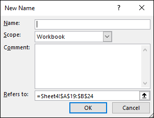
FIGURE 3-1: Creating a named area with the New Name dialog box.

Named areas are easily referenced in formulas. For example, if a workbook contains a named area Sales, the values of all the cells in Sales can be summed up like this:

=SUM(Sales)

Assume that Sales contains three cells with these values: 10, 15, and 20. These values, of course, can be entered directly in the SUM function like this:

=SUM(10,15,20)

This is almost an array, but not quite. Excel recognizes a group of values to be an array when they are enclosed in braces ({ and }). Therefore, to enter the array of values into the function, you make an entry that looks like this:

=SUM({10,15,20})

Essentially the braces tell Excel to treat the group of values as an array. So far, you may be wondering about the usefulness of an array, but in the next section, I show you how using arrays with standard functions such as SUM can provide sophisticated results.

To enter values as an array within a function, enclose them in braces. Braces have a curly look and are not to be confused with brackets. On a typical keyboard, braces and brackets are on the same key. Holding the Shift key while pressing the brace/bracket key provides the brace.

However, getting the braces into the formula takes a particular keystroke. You don't type braces directly.

Using Arrays in Formulas

You can use arrays when entering formulas and functions. Typically, the arguments to a function are entered in a different manner, which I demonstrate in this section. Using arrays can save entry steps and deliver an answer in a single formula. This is useful in situations that normally require a set of intermediate calculations from which the final result is calculated. I don’t know about you, but I like shortcuts, especially when I have too much to do!

Here’s an example: The SUM function is normally used to add a few numbers together. Summing up a few numbers doesn’t require an array formula per se, but what about summing up the results of other calculations? This next example shows how using an array simplifies getting to the final result.

Figure 3-2 shows a small portfolio of stocks. Column A has the stock symbols, column B has the number of shares per stock, and column C has a recent price for each stock.

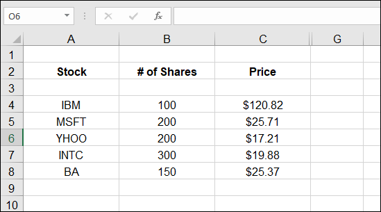
FIGURE 3-2: A stock portfolio.

The task is to find out the total value of the portfolio. The typical way to do this is to

1. Multiply the number of shares for each stock by its price.
2. Sum up the results from Step 1.

Figure 3-3 shows a common way to do this. Column D contains formulas to calculate the value of each stock in the portfolio. This is done by multiplying the number of shares for each stock by its price. For example, cell D4 contains the formula =B4*C4. Cell D10 sums up the interim results with the formula =SUM(D4:D8).

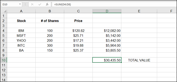
FIGURE 3-3: Calculating the value of a stock portfolio the old-fashioned way.

The method shown in Figure 3-3 requires creating additional calculations — those in column D. These calculations are necessary if you need to know the value of each stock, but not if all you need to know is the value of the portfolio as a whole.

Fortunately, alternatives to this standard approach exist. One is to embed the separate multiplicative steps directly in the SUM function, like this:

=SUM(B4*C4,B5*C5,B6*C6,B7*C7,B8*C8)

That works, but it's bloated, to say the least. What if you had 20 stocks in the portfolio? Forget it!

Another alternative is the SUMPRODUCT function. This function sums the products, just as the other methods shown here do. The limitation, however, is that SUMPRODUCT can be used only for summing. It cannot, for example, give you an average.

In many situations such as this one, your best bet is to use an array function. Figure 3-4 shows the correct result from using the SUM function entered as an array function. Notice that the formula in the Formula Bar begins and ends with a brace.

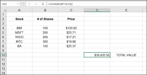
FIGURE 3-4: Calculating the value of a stock portfolio using an array function.

The syntax is important. Two ranges are entered in the function: One contains the cells that hold the number of shares, and the other contains the cells that have the stock prices. These are multiplied in the function by entering the multiplication operator (*):

{=SUM(B4:B8*C4:C8)}

Ctrl+Shift+Enter had been pressed to turn the whole thing into an array function. You use that special keystroke combination when you finish the formula, not before. Note the lack of subtotals (per stock) in cells D4:D8. Compare Figure 3-4 with Figure 3-3, and you can see the difference.

Use Ctrl+Shift+Enter to turn a formula into an array formula. You must use the key combination after entering the formula instead of pressing Enter. The key combination takes the place of pressing Enter.

Here’s how you use an array with the SUM function:

1. Enter two columns of values.

   The two lists must be the same size.

2. Position the cursor in the cell where you want the result to appear.

3. Type =SUM( to start the function.

   Note that a brace is not entered in this step.

4. Click the first cell in the first list, hold the left mouse button down, drag the pointer over the first list, and then release the mouse button.
5. Type the multiplication sign (*).
6. Click the first cell of the second list, hold down the left mouse button, and drag the pointer over the second list.
7. Release the mouse button.
8. Type a ).

9. Press Ctrl+Shift+Enter to end the function.

   Do not just press Enter by itself when using an array with the SUM function.

Array functions are useful for saving steps in mathematical operations. Therefore, you can apply these examples to a number of functions, such as AVERAGE, MAX, MIN, and so on.

As another example, suppose that you run a fleet of taxis, and you need to calculate the average cost of gasoline per mile driven. This is easy to calculate for a single vehicle. You just divide the total spent on gasoline by the total miles driven for a given period of time. The calculation looks like this:

cost of gasoline per mile = total spent on gasoline ÷ total miles driven

How can you easily calculate this for a fleet of vehicles? Figure 3-5 shows how this is done. The vehicles are listed in column A, the total miles driven for the month appear in column B, and the total amounts spent on gasoline appear in column C.

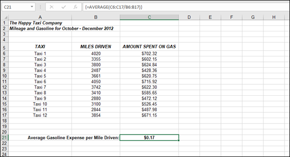
FIGURE 3-5: Making an easy calculation using an array formula.

One single formula in cell C21 answers the question. When you use the AVERAGE function in an array formula, the result is returned without the need for any intermediate calculations. The formula looks like this:

{=AVERAGE(C6:C17/B6:B17)}

Working with Functions That Return Arrays

A few functions actually return arrays of data. Instead of providing a single result, as most functions do, these functions return several values. The number of actual returned values is directly related to the function’s arguments. The returned values go into a range of cells.

Excel array functions accept arrays as arguments and possibly return arrays of data.

A good example of this is the TRANSPOSE function. This interesting function is used to reorient data. Data situated a given way in columns and rows is transposed (changed to be presented instead in rows and columns). Figure 3-6 shows how this works.

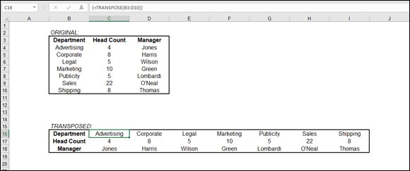
FIGURE 3-6: Transposing data.

Cells B3 through D10 contain information about departments in a company. Departments are listed going down column B. Note that the area of B3 through D10 specifically occupies three columns and eight rows. The header row is included in the area.

Cells B16 through I18 contain the transposed data. It is the same data, but now it occupies eight columns and three rows. In total number of cells, this is the same size as the original area. Just as important is that the area is made up of the same dimensions, just reversed. That is, a 3-by-8 area became an 8-by-3 area. The number of cells remains 24. However, the transposed area has not been altered to be 6 by 4, 2 by 12, or any other two dimensions that cover 24 cells.

Every single cell in the B16:I18 range contains the same formula: {=TRANSPOSE(B3:D10)}. However, the function was entered only once.

In detail, here is how you can use the TRANSPOSE function:

1. Enter some data that occupies at least two adjacent cells.

   Creating an area of data that spans multiple rows and columns is best for seeing how useful the function is.

2. Elsewhere on the worksheet, select an area that covers the same number of cells but has the length of the sides of the original area reversed.

   For example:

   • If the original area is 2 columns and 6 rows, select an area that is 6 columns and 2 rows.
   • If the original area is 1 column and 2 rows, select an area that is 2 columns and 1 row.
   • If the original area is 200 columns and 201 rows, select an area that is 201 columns and 200 rows.
   • If the original area is 5 columns and 5 rows, select an area that is 5 columns and 5 rows. (A square area is transposed into a square area.)

   Figure 3-7 shows an area of data and a selected area ready to receive the transposed data. The original data area occupies 11 columns and 3 rows. The selected area is 3 columns by 11 rows.

3. Type =TRANSPOSE( to start the function.

   Because the receiving area is already selected, the entry goes into the first cell of the area.

4. Click the first cell in the original data, drag the pointer over the entire original data area while keeping the mouse button down, and release the mouse button when the area is selected.

   The function now shows the range of the original area. Figure 3-8 shows how the entry should appear at this step.

5. Type ).
6. Press Ctrl+Shift+Enter to end the function.

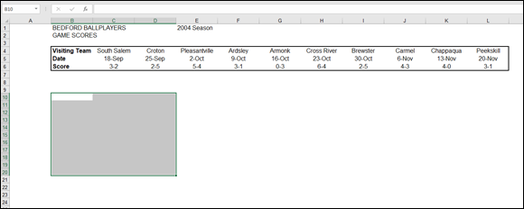
FIGURE 3-7: Preparing an area to receive transposed data.

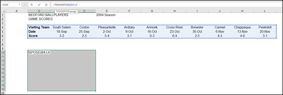
FIGURE 3-8: Completing the function.

Note that the transposed data does not necessarily take on the formatting of the original area. You may need to format the area. Figure 3-9 shows the result of using TRANSPOSE and then formatting the transposed data.

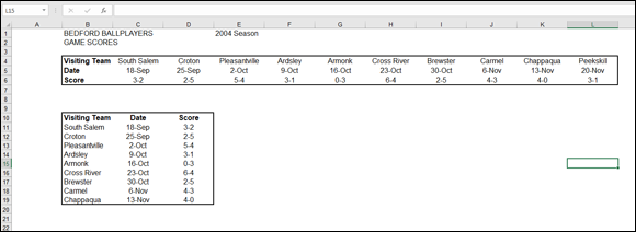
FIGURE 3-9: Transposed data after formatting.

Wait! Isn’t this a waste of time? Excel can easily transpose data when you use the Paste Special dialog box. Simply copying a range of data and using this dialog box to paste the data gives the same result as the TRANSPOSE function. Or does it?

Figure 3-10 shows the Paste Special dialog box with the Transpose check box selected. This option transposes the data. You don’t even have to select the correct number of rows and columns where the transposed data will land. It just appears transposed, with the active cell as the corner of the area.

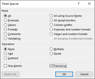
FIGURE 3-10: Using the Paste Special dialog box to transpose data.

However, when data is transposed with the Paste Special dialog box, the actual data is copied to the new area. By contrast, the TRANSPOSE function pastes a formula that references the original data — and that is the key point. When data is changed in the original area, the change is reflected in the new, transposed area if the TRANSPOSE function was used.

You can transpose data in two ways. The area filled with the TRANSPOSE function references the original data and will update as original data is changed. Using the Paste Special dialog box to transpose data creates values that do not update when the original data changes.