Chapter 6

Appreciating What You’ll Get, Depreciating What You’ve Got

IN THIS CHAPTER

Determining what an investment is worth

Using different depreciation methods

Evaluating business opportunities

Money makes the world go ’round, so the saying goes. I have a new one: Excel functions make the money go ’round. Excel has functions that let you figure out what an investment will be worth at a future date. We all know it’s a good thing to look for a good interest rate on an investment. With the FV (Future Value) function, you can take this a step further and know how much the investment will be worth down the road.

Have you ever wondered what to do with some extra money? You can put it in the bank, you can pay off a debt, or you can purchase something. Excel helps you figure out the best course of action by using the IRR (Internal Rate of Return) function. The IRR function lets you boil down each option to a single value that you can then use to compare opportunities and select the best one.

For the business set, Excel has a number of functions to help create depreciation schedules. Look no further than the SLN, SYD, DB, and DDB functions for help in this area. Brush up on these, and you can talk shop with your accountant!

SLN is a function used to calculate straight-line deprecation. SYD is a function to calculate sum-of-years’-digits depreciation. DB and DDB are variations of the declining-balance method of depreciation.

Looking into the Future

The FV function tells you what an investment will be worth in the future. The function takes an initial amount of money and also takes into account additional periodic fixed payments. You also specify a rate of return — the interest rate — and the returned value tells you what the investment will be worth after a specified period of time.

For example, you start a savings account with a certain amount, say $1,000. Every month you add $50 to the account. The bank pays an annual interest rate of 5 percent. At the end of 2 years, what is value of the account?

This is the type of question the FV function answers. The function takes five arguments:

• Interest rate: This argument is the annual interest rate. When entered in the function, it needs to be divided by the number of payments per year — presumably 12, if the payments are monthly.
• Number of payments: This argument is the total number of payments in the investment. These payments are the ones beyond the initial investment; don’t include the initial investment in this figure. If payments occur monthly and the investment is for 3 years, there are 36 payments.
• Payment amount: This argument is the fixed amount contributed to the investment each payment period.
• Initial investment (also called PV or present value): This argument is the amount the investment starts with. A possible value is 0, which means no initial amount is used to start the investment. This is an optional argument. If left out, 0 is assumed.
• How payments are applied: The periodic payments may be applied at either the beginning of each period or the end of each period. This argument affects the result to a small but noticeable degree. Either a 0 or a 1 can be entered. A 0 tells the function that payments occur at the end of the period. A 1 tells the function that payments occur at the start of the period. This is an optional argument. If it’s left out, 0 is assumed.

When using the FV function, be sure to enter the initial investment amount and the periodic payment amount as negative numbers. Although you’re investing these monies, you’re essentially paying out (even if it’s into your own account). Therefore, these are cash flows out.

Here’s how to use the FV function:

1. Enter the following data in separate cells of the worksheet:

   • Annual interest rate
   • Number of payment periods
   • Periodic payment amount
   • Initial investment amount

   You can add labels to adjacent cells to identify the values, if desired.

2. Position the cursor in the cell where you want the results to appear.
3. Type =FV( to begin the function entry.
4. Click the cell where you entered the annual interest rate, or enter the cell address.
5. Type /12 to divide the annual interest rate to get the monthly interest rate.
6. Type a comma (,).
7. Click the cell where you entered the total number of payments, or enter the cell address.
8. Type a comma (,).
9. Click the cell where you entered the periodic payment amount, or enter the cell address.
10. Type a comma (,).
11. Click the cell where you entered the initial investment amount, or enter the cell address.
12. (Optional) Type a comma (,) and then type either 0 or 1 to identify whether payments are made at the beginning of the period (0) or at the end of the period (1).
13. Type a ) and press Enter.

Figure 6-1 shows how much an investment is worth after 2 years. The investment is begun with $1,000, and $50 is added each month. The interest rate is 5 percent. The value of the investment at the end is $2,364.24. The actual layout was $2,200 ($1,000 + [$50 × 24]). The account has earned $164.24.

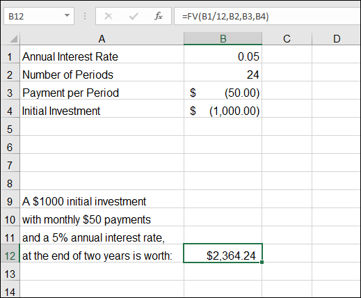
FIGURE 6-1: Earning extra money in an investment.

Depreciating the Finer Things in Life

Depreciation is the technique of allocating the cost of an asset over the useful period that the asset is used. Depreciation is applied to capital assets, which are tangible goods that provide usefulness for a year or more.

Vehicles, buildings, and equipment are the types of assets that depreciation can be applied to. A tuna sandwich is not a capital asset because its usefulness is going to last for just the few minutes it takes someone to eat it — although the person eating it may expect to capitalize on it!

Take the example of a business purchasing a delivery truck. The truck costs $35,000. It’s expected to be used for 12 years; this is known as the life of the asset. At the end of 12 years, the vehicle’s estimated worth will be $8,000. These figures follow certain terminology used in the depreciation formulas:

• Cost: This is the initial cost of the item ($35,000). This could include not just the price of the item, but also costs associated with getting and installing the item, such as delivery costs.
• Salvage: This is the value of the item at the end of the useful life of the item ($8,000).
• Life: This is the number of periods that the depreciation is applied to. This is usually expressed in years (in this case, 12 years).

Depreciation is calculated in different ways. Some techniques assume that an asset provides the majority of its usefulness during the early periods of its life. Depreciation in this case is applied on a sliding scale from the first period to the last. The bulk of the depreciation gets applied in the first few periods. This is known as an accelerated depreciation schedule. Sometimes, the depreciation amount runs out sooner than the asset’s life. Alternatively, depreciation can be applied evenly over all the periods. In this case, each period of the asset’s life has an equal amount of depreciation to apply. The different depreciation methods are summarized in Table 6-1.

TABLE 6-1 Depreciation Methods

Method	Comments	Excel Function That Uses the Method
Straight Line	Evenly applies the depreciable cost (Cost – Salvage) among the periods. Uses the formula (Cost – Salvage) ÷ Number of Periods.	SLN
Sum of Years’ Digits	First sums up the periods, literally. For example, if there are five periods, the method first calculates the sum of the years’ digits as 1 + 2 + 3 + 4 + 5 = 15. This method creates an accelerated depreciation schedule. See Excel Help for more information.	SYD
Double Declining Balance	Creates an accelerated depreciation schedule by doubling the straight-line depreciation rate but then applies it to the running declining balance of the asset cost, instead of to the fixed depreciable cost.	DDB, DB

The depreciable cost is the original cost minus the salvage value.

Figure 6-2 shows a worksheet with a few different methods. The methods use the example of a delivery truck that costs $35,000, is used for 12 years, and has an ending value of $8,000. An important calculation in all these methods is the depreciable cost, which is the original cost minus the salvage value. In this example, the depreciable cost is $27,000, calculated as $35,000 – $8,000.

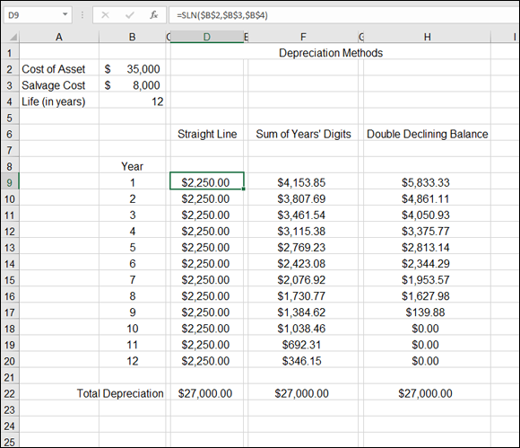
FIGURE 6-2: Depreciating an asset.

In the three depreciation methods shown in Figure 6-2 — Straight Line, Sum of Years’ Digits, and Double Declining Balance — all end with the accumulated depreciation at the end of life equal to the depreciable cost, or the cost minus the salvage.

However, each method arrives at the total in a different way. The Straight Line method simply applies an even amount among the periods. The Sum of Years’ Digits and Double Declining Balance methods accelerate the depreciation. In fact the Double Declining Balance method does it to such a degree that all the depreciation is accounted for before the asset’s life is over.

Calculating straight-line depreciation

The SLN function calculates the depreciation amount for each period of the life of the asset. The arguments are simple: just the cost, salvage, and the number of periods. In Figure 6-2, each cell in the range D9:D20 has the same formula: =SLN($B$2,$B$3,$B$4). Because straight-line depreciation provides an equal amount of depreciation to each period, it makes sense that each cell uses the formula verbatim. The answer is the same regardless of the period. (This approach differs from the accelerated depreciation methods that follow.)

Using dollar signs ($) in front of column and row indicators fixes the cell address so it won't change.

Here’s how to use the SLN function:

1. Enter three values in a worksheet:
   • Cost of an asset
   • Salvage value (always less than the original cost)
   • Number of periods in the life of the asset (usually, years)
2. Type =SLN( to begin the function entry.
3. Click the cell that has the original cost, or enter its address.
4. Type a comma (,).
5. Click the cell that has the salvage amount, or enter its address.
6. Type a comma (,).
7. Click the cell that has the number of periods, or enter its address.
8. Type a ) and press Enter.

The returned value is the amount of depreciation per period. Each period has the same depreciation amount. The same formula, referencing the same cells (using $ for absolute referencing), is in each cell in the D9:D20 range.

Creating an accelerated depreciation schedule

The SYD function creates an accelerated depreciation schedule (that is, more depreciation is applied in the early periods of the asset’s life). The method uses an interesting technique of first summing up the years’ digits. So for a depreciation schedule that covers 5 years, a value of 15 is first calculated as 1 + 2 + 3 + 4 + 5 = 15. If the schedule is for 10 years, the first step of the method is to calculate the sum of the digits 1 through 10, like this: 1 + 2 + 3 + 4 + 5 + 6 + 7 + 8 + 9 + 10 = 55.

Then the years’-digit sum is used as the denominator in calculations with the actual digits themselves to determine a percentage per period. The digits in the calculations are the reverse of the actual periods. In other words, in a 5-year depreciation schedule, the depreciation for the first period is calculated as (5 ÷ 15) × Depreciable Cost. The second-period depreciation is calculated as (4 ÷ 15) × Depreciable Cost. The following table makes it clear, with an assumed 5-year depreciation on a depreciable cost of $6,000, and a salvage value of $0:

Period	Calculation	Result
1	() × 6,000	$2,000
2	() × 6,000	$1,600
3	() × 6,000	$1,200
4	() × 6,000	$800
5	() × 6,000	$400

Guess what? You don’t even need to know how this works! Excel does all the figuring for you. The SYD function takes four arguments: the cost, the salvage, the life (the number of periods), and the period to be calculated.

SYD returns the depreciation for a single period. Earlier in this chapter, I show you that the SLN function also returns the depreciation per period, but because all periods are the same, the SLN function doesn’t need to have an actual period entered as an argument.

The SYD function returns a different depreciation amount for each period, so the period must be entered as an argument. In Figure 6-2, each formula in the range F9:F20 uses the SYD function but has a different period as the fourth argument. For example, cell F9 has the formula =SYD($B$2,$B$3,$B$4,B9), and cell F10 has the formula =SYD($B$2,$B$3,$B$4,B10). The last argument provides a different value.

Here's how to use the SYD function to calculate the depreciation for one period:

1. Enter three values in a worksheet:
   • Cost of an asset
   • Salvage value (always less than the original cost)
   • Number of periods in the life of the asset (usually, years)
2. Type =SYD( to begin the function entry.
3. Click the cell that has the original cost, or enter its address.
4. Type a comma (,).
5. Click the cell that has the salvage amount, or enter its address.
6. Type a comma (,).
7. Click the cell that has the number of periods, or enter its address.
8. Type a comma (,).
9. Enter a number for the period for which to calculate the depreciation.
10. Type a ) and press Enter.

The returned value is the amount of depreciation for the entered period. To calculate the depreciation for the entire set of periods, enter a formula with the SYD function in the same number of cells as there are periods. In this case, each cell has a different period entered for the fourth argument. To make this type of entry easy to do, enter the first three arguments as absolute cell addresses. In other words, use the dollar sign ($) in front of the row and column indicators. Leave the fourth argument in the relative address format.

In cell F9 in Figure 6-2, the formula is =SYD($B$2,$B$3,$B$4,B9). Note that the first three arguments are fixed to the cells B2, B3, and B4. With this formula entered in cell F9, simply dragging the formula (using the fill handle in the lower-right corner of the cell) down to F20 fills the range of cells that need the calculation. The fourth argument changes in each row. For example, cell F20 has this formula: =SYD($B$2,$B$3,$B$4,B20).

Creating an even faster accelerated depreciation schedule

The Double Declining Balance method provides an accelerated depreciation schedule but calculates the amounts differently from the Sum of Years' Digits method.

Although rooted in the doubling of the Straight Line method (which is not an accelerated method), the calculation for each successive period is based on the remaining value of the asset after each period instead of to the depreciable cost. Because the remaining value is reduced each period, the schedule for each period is different.

The DDB function takes five arguments. The first four are required:

• Cost
• Salvage
• Life (the number of periods)
• Period for which the depreciation is to be calculated

The fifth argument is the factor. A factor of 2 tells the function to use the Double Declining Balance method. Other values can be used, such as 1.5. The factor is the rate at which the balance declines. A smaller value (than the default of 2) results in a longer time for the balance to decline. When the fifth argument is omitted, the value of 2 is the default.

The DDB function returns a different depreciation amount for each period, so the period must be entered as an argument. In Figure 6-2, each formula in the range H9:H20 uses the DDB function but has a different period as the fourth argument. For example, cell H9 has the formula =DDB($B$2,$B$3,$B$4,B9) and cell H10 has the formula =DDB($B$2,$B$3,$B$4,B10). The last argument provides a different value.

As shown in Figure 6-2 earlier in this chapter, the Double Declining Balance method provides an even more accelerated depreciation schedule than the Sum of Years' Digits method does. In fact, the depreciation is fully accounted for before the asset has reached the end of its life.

Here’s how to use the DDB function to calculate the depreciation for one period:

1. Enter three values in a worksheet:
   • Cost of an asset
   • Salvage value (always less than the original cost)
   • Number of periods in the life of the asset (usually, years)
2. Type =DDB( to begin the function entry.
3. Click the cell that has the original cost, or enter its address.
4. Type a comma (,).
5. Click the cell that has the salvage amount, or enter its address.
6. Type a comma (,).
7. Click the cell that has the number of periods.
8. Type a comma (,).
9. Enter a number for the period for which to calculate the depreciation.
10. If a variation on the Double Declining Balance method is desired, enter a comma (,) and a value other than 2.
11. Type a ) and press Enter.

The returned value is the amount of depreciation for the entered period. To calculate the depreciation for the entire set of periods, you need to enter a formula with the DDB function in the same number of cells as there are periods. In this case, each cell would have a different period entered for the fourth argument. One of the best approaches is to use absolute addressing for the first three function arguments. Then, when you fill the rest of the cells by dragging or copying, the references to original cost, salvage amount, and number of periods stay constant. You can see an example of absolute addressing in the Formula Bar in Figure 6-2.

There is no hard-and-fast rule for selecting the best depreciation method. However, it makes sense to use one that matches the depreciating value of the asset. For example, cars lose a good deal of their value in the first few years, so applying an accelerated depreciation schedule makes sense.

Calculating a midyear depreciation schedule

Most assets are not purchased, delivered, and put into service on January 1. Excel provides a depreciation formula, DB, that accounts for the periods being offset from the calendar year. The DB function takes five arguments. The first four are the typical ones: the cost, the salvage, the life (the number of periods), and the period for which the depreciation is to be calculated. The fifth argument is the number of months in the first year. The fifth argument is optional; when it's left out, the function uses 12 as a default.

For the fifth argument, a value of 3 means the depreciation starts in October (October through December is 3 months), so the amount of depreciation charged in the first calendar year is small. A value of 11 means that the depreciation starts in February (February through December is 11 months).

Figure 6-3 shows a depreciation schedule created with the DB function. Note that the life of the asset is 12 years (in cell B4) but that the formula is applied to 13 different periods. Including an extra year is necessary because the first year is partial. The remaining months must spill into an extra calendar year. The depreciation periods and the calendar years are offset.

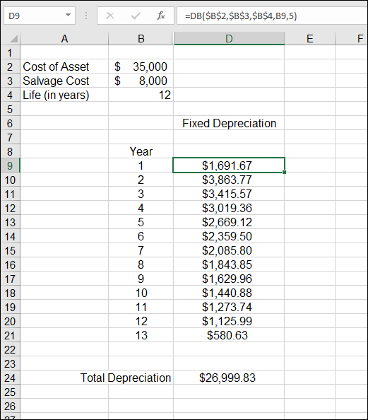
FIGURE 6-3: Offsetting depreciation periods from the calendar.

The example in Figure 6-3 is for an asset put into service in August. Cell D9 has the formula =DB($B$2,$B$3,$B$4,B9,5). The fifth argument is 5, which indicates that the first-year depreciation covers 5 months: August, September, October, November, and December.

Here’s how to use the DB function to calculate the depreciation for one period:

1. Enter three values in a worksheet:
   • Cost of an asset
   • Salvage value (always less than the original cost)
   • Number of periods in the life of the asset (usually, years)
2. Type =DB( to begin the function entry.
3. Click the cell that has the original cost, or enter its address.
4. Type a comma (,).
5. Click the cell that has the salvage amount, or enter its address.
6. Type a comma (,).
7. Click the cell that has the number of periods.
8. Type a comma (,).
9. Enter a number for the period for which to calculate the depreciation.
10. Type a comma (,).
11. Enter the number of months within the first year that the depreciation is applied to.
12. Type a ) and press Enter.

The returned value is the amount of depreciation for the entered period. To calculate the depreciation for the entire set of periods, you need to enter a formula with the DB function in the same number of cells as there are periods. However, you should make space for an additional period (refer to Figure 6-3).

Enter the constant arguments of the function with absolute addressing (the dollar signs used in front of row numbers or column letters). This makes the function easy to apply across multiple cells by copying the formula. The references to the pertinent function arguments stay constant.

Measuring Your Internals

Which is better to do: pay off your credit card or invest in Uncle Ralph’s new business venture? You’re about to finance a car. Should you put down a large down payment? Or should you put down a small amount and invest the rest? How can you make decisions about alternative financial opportunities like these?

The Internal Rate of Return (IRR) method helps answer these types of questions. The IRR function analyzes the cash flows in and out of an investment and calculates an interest rate that is the effective result of the cash flows. In other words, all the various cash flows are accounted for, and one interest rate is returned. Then you can compare this figure with other financial opportunities.

Perhaps Uncle Ralph’s business venture will provide a 10 percent return on your investment. On the other hand, the credit card company charges you 12 percent on your balance. In this case, paying off the credit card is wiser. Why? Because earning 10 percent is pointless when you’re just losing 12 percent elsewhere. Uncle Ralph will understand, won’t he?

The IRR function takes two arguments. The first is required; the second is optional in some situations and required in others.

The first argument is an array of cash flows. Following the cash-flows standard, money coming in is entered as a positive value, and money going out is entered as a negative value. Assuming that the particular cash flows in and out are entered on a worksheet, the first argument to the function is the range of cells.

The second argument is a guess at what the result should be. I know this sounds crazy, but Excel may need your help here (though most times, it won’t). The IRR function works by starting by guessing the result and calculating how closely the guess matches the data. Then it adjusts the guess up or down and repeats the process (a technique called iteration) until it arrives at the correct answer. If Excel doesn’t figure it out in 20 tries, the #NUM! error is returned. In this case, you could enter a guess in the function to help it along. For example, 0.05 indicates a guess of 5 percent, 0.15 indicates a guess of 15 percent, and so on. You can enter a negative number, too. For example, entering –0.05 tells the function that you expect a 5 percent loss. If you don't enter a guess, Excel assumes 0.1 (10 percent).

Figure 6-4 shows a business venture that has been evaluated with IRR. The project is to create and market t-shirts. Assorted costs such as paying artists are cash flows out, entered as negative numbers. The one positive value in cell B7 is the expected revenue.

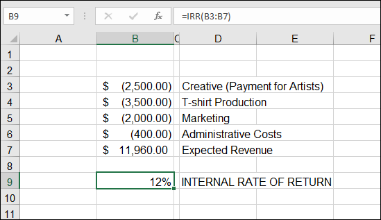
FIGURE 6-4: Calculating the return on a business venture.

The IRR function has been used to calculate an expected rate of return. The formula in cell B10 is =IRR(B3:B7). The entered range includes all the cash flows, in and out.

This project has an internal rate of return of 12 percent. By the way, the investment amount in this case is the sum of all the cash flows out: $8,400. Earning back $11,960 makes this a good investment. The revenue is significantly higher than the outlay.

Even though a business opportunity seems worthy after IRR has been applied, you must consider other factors. For example, you may have to borrow the money to invest in the business venture. The real number to look at is the IRR of the business venture less the cost of borrowing the money to invest.

However, the project can now be compared with other investments. Another project may calculate to a higher internal rate of return. Then the second project would make sense to pursue. Of course, don’t forget the fun factor. Making t-shirts may be worth giving up a few extra points!

When you’re comparing opportunities with the IRR function, a higher returned value is a better result than a lower IRR.

Figure 6-5 compares the business venture in Figure 6-4 with another investment opportunity. The second business venture is a startup videography business for weddings and other affairs. There is a significant outlay for equipment and marketing. An internal rate of return is calculated for the first year, and then for the first and second year together. Cell H10 has the formula =IRR(H3:H5), and cell H11 has the formula =IRR(H3:H6). It's clear that even within the first year, the second business venture surpasses the first.

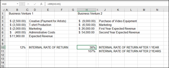
FIGURE 6-5: Comparing business opportunities.

This is how to use the IRR function:

1. Enter a series of cash-flow values:
   • Money paid out, such as the initial investment, as a negative value
   • Money coming in, such as revenue, as a positive value
2. Type =IRR( to begin the function entry.
3. Drag the cursor over the range of cells containing the cash flows, or enter the range address.

4. Optionally, enter a guess to help the function.

   To do this, type a comma (,) and then enter a decimal value to be used as a percentage (such as 0.2 for 20 percent). You can enter a positive or negative value.

5. Type a ) and press Enter.

Considering that IRR is based on cash flows, in and out, it’s prudent to include paying yourself, as well as accounting for investments back in the business. Salary is cash flow out; investment is cash flow in.

Figure 6-6 expands on the videography business with a detailed example. As a business, it has various cash flows in and out — investment, utility payments, professional fees (to the accountant and lawyer), advertising, salary, and so on.

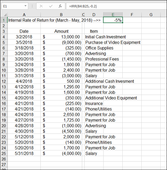
FIGURE 6-6: Calculating IRR with several cash flows.

The internal rate of return for the first 3 months of the business is displayed in cell E1. The formula is =IRR(B4:B25,-0.2). By the way, this one needed a guess to return the answer. The guess is –0.2. The internal rate or return is –5 percent. The videography business is not a moneymaker after a few months, but this is true of many startups.

Note that this example includes dates. The IRR function works with an assumption that cash flows are periodic, which they aren’t in this example. Another function, XIRR, handles dates in its calculation of the internal rate of return.