Chapter 8

Advancing Your Math

IN THIS CHAPTER

Calculating the circumference, diameter, and area of a circle

Returning random numbers

Working with combinations and permutations

Performing sophisticated multiplication

Using the MOD function to test other numerical values

Using the SUBTOTAL function for a variety of arithmetic and statistical totals

Using the SUMIF and SUMIFS functions for selective summation

Getting an angle on trigonometry functions

In this chapter, I show you some of the more advanced math functions. You won’t use these functions every day, but they’re just the right thing when you need them. Some of this will come back to you because you probably learned most of this in school.

Using PI to Calculate Circumference and Diameter

Pi is the ratio of a circle’s circumference to its diameter. A circle’s circumference is its outer edge and is equal to the complete distance around the circle. A circle’s diameter is the length of a straight line running from one side of the circle, through the middle, and reaching the other side.

Dividing a circle’s circumference by its diameter returns a value of approximately 3.14159, known as pi. Pi is represented with the Greek letter pi and the symbol π.

Mathematicians have proved that pi is an irrational number — in other words, that it has an infinite number of decimal places. They have calculated the value of pi to many thousands of decimal places, but you don’t need that level of precision in most calculations. Many people use the value 3.14159 for pi, but the PI function in Excel does a bit better than that. Excel returns a value of pi accurate to 15 digits — that is 14 decimal places in addition to the integer 3. This function has no input arguments. The function uses this syntax:

=PI()

In Excel, the PI function always returns 3.14159265358979, but initially, it may look like some of the digits after the decimal point are missing. Change the formatting of the cell to display numbers with 14 decimal places to see the entire number.

If you know the circumference of a circle, you can calculate its diameter with this formula:

diameter = circumference ÷ pi

If you know the diameter of a circle, you can calculate its circumference with this formula:

circumference = diameter × pi

If you know the diameter of a circle, you can calculate the area of the circle. A component of this calculation is the radius, which equals one half of the diameter. The formula is

area = (diameter × 0.5)^2 × pi

Generating and Using Random Numbers

Random numbers are, by definition, unpredictable. That is, given a series of random numbers, you can’t predict the next number from what has come before. Random numbers are quite useful for trying formulas and calculations. Suppose that you’re creating a worksheet to perform various kinds of data analysis. You may not have any real data yet, but you can generate random numbers to test the formulas and charts in the worksheet.

For example, an actuary may want to test some calculations based on a distribution of people’s ages. Random numbers between 18 and 65 can be used for this task. You don’t have to manually enter fixed values between 18 and 65, because Excel can generate them automatically via the RAND function.

The all-purpose RAND function

The RAND function is simple; it takes no arguments and returns a decimal value between 0 and 1. That is, RAND never actually returns 0 or 1; the value is always in between these two numbers. The function is entered like this:

=RAND()

The RAND function returns values such as 0.136852731, 0.856104058, or 0.009277161. “Yikes!” you may be thinking. “How do these numbers help if you need values between 18 and 65?” Actually, it's easy with a little extra math.

There is a standard calculation for generating random numbers within a determined range. The calculation follows:

= RAND() * (high number - low number) + low number

Using 18 and 65 as a desired range of numbers, the formula looks like =RAND()*(65-18)+18. Some sample values returned with this formula follow:

• 51.71777896
• 27.20727871
• 24.61657068
• 55.27298686
• 49.93632709
• 43.60069745

Almost usable! But what about the long decimal portions of these numbers? Some people lie about their ages, but I've never heard someone say he’s 27.2 years old!

All that is needed now for this 18-to-65 age example is to include the INT or ROUND function. INT simply discards the decimal portion of a number. ROUND allows control of how to handle the decimal portion.

The syntax for using the INT function with the RAND function follows:

= INT((high number – low number + 1) * RAND() + low number)

The syntax for using the ROUND function with the RAND function follows:

=ROUND(RAND() * (high number-low number) + low number,0)

Try it yourself! Here’s how to use RAND and INT together:

1. Position the pointer in the cell where you want the results displayed.
2. Type =INT(( to begin the formula.
3. Click the cell that has the highest number to be used, or enter such a value.
4. Type – (a minus sign).
5. Click the cell that has the lowest number to be used, or enter such a value.
6. Type +1) * RAND( ) + .
7. Again, click the cell that has the lowest number to be used, or enter the value.
8. Type a ) and press Enter.

A random number, somewhere in the range between the low and high number, is returned.

Table 8-1 shows how returned random numbers can be altered with the INT and ROUND functions.

TABLE 8-1 Using INT and ROUND to Process Random Values

Value	Value Returned with INT	Value Returned with ROUND
51.71777896	51	52
27.20727871	27	27
24.61657068	24	25
55.27298686	55	55
49.93632709	49	50
43.60069745	43	44

Table 8-1 points out how the INT and ROUND functions return different numbers. For example, 51.71777896 is more accurately rounded to 52. Bear in mind that the second argument in the ROUND function, 0 in this case, has an effect on how the rounding works. A 0 tells the ROUND function to round the number to the nearest integer, up or down to whichever integer is closest to the number.

Random values are volatile. Each time a worksheet is recalculated, the random values change. You can prevent this behavior by typing the formula directly in the Formula Bar, pressing the F9 key, and then pressing Enter.

A last but not insignificant note about using the RAND function: It is subject to the recalculation feature built into worksheets. In other words, each time the worksheet calculates, the RAND function is rerun and returns a new random number. The calculation setting in your worksheet is probably set to automatic. You can check this by looking at the Formulas tab of the Excel Options dialog box. Figure 8-1 shows the calculation setting. On a setting of Automatic, the worksheet recalculates with every action. The random generated numbers keep changing, which can become quite annoying if this is not what you intended to have happen. However, I bet you did want the number to change; otherwise, why use something “random” in the first place?

FIGURE 8-1: Setting worksheet calculation options.

Luckily, you can generate a random number but have it remain fixed regardless of the calculation setting. The method is to type the RAND function, along with any other parts of a larger formula, directly in the Formula Bar. After you type your formula, press the F9 key and then press Enter. This tells Excel to calculate the formula and enter the returned random number as a fixed number instead of a formula. If you press Enter or finish the entry in some way without pressing the F9 key, you have to enter it again.

Precise randomness with RANDBETWEEN

Using the RAND function returns a value between 0 and 1, and when you use it with other functions, such as ROUND, you can get a random number within a range that you specify. If you just need a quick way to get an integer (no decimal portion!) within a given range, use RANDBETWEEN.

The RANDBETWEEN function takes two arguments: the low and high numbers of the desired range. It works only with integers. You can put real numbers in the range, but the result will still be an integer.

To use RANDBETWEEN, follow these steps:

1. Position the pointer in the cell where you want the results displayed.
2. Type =RANDBETWEEN( to begin the formula.
3. Click the cell that has the low number of the desired range, or enter such a value.
4. Type a comma (,).
5. Click the cell that has the highest number of the desired range, or enter such a value.
6. Type a ) and press Enter.

For example, =RANDBETWEEN(10,20) returns a random integer between 10 and 20.

Ordering Items

Remember the Beatles? John, Paul, George, and Ringo? If you’re a drummer, you may think of the Beatles as Ringo, John, Paul, and George. The order of items in a list is known as a permutation. The more items in a list, the more possible permutations exist.

Excel provides the PERMUT function. It takes two arguments: the total number of items to choose among and the number of items to be used in determining the permutations. The function returns a single whole number. The syntax of the function follows:

=PERMUT(total number of items, number of items to use)

Use permutations when the order of items is important.

The total number of items must be the same as or greater than the number of items to use; otherwise, an error is generated.

You may be confused about why the function takes two arguments. On the surface, it seems that the first argument is sufficient. Well, not quite. Getting back to the Beatles, anyone have a copy of Abbey Road I can borrow? If we plug in 4 as the number for both arguments

=PERMUT(4,4)

Twenty-four permutations are returned:

• John Paul George Ringo
• John Paul Ringo George
• John George Paul Ringo
• John George Ringo Paul
• John Ringo Paul George
• John Ringo George Paul
• Paul John George Ringo
• Paul John Ringo George
• Paul George John Ringo
• Paul George Ringo John
• Paul Ringo John George
• Paul Ringo George John
• George John Paul Ringo
• George John Ringo Paul
• George Paul John Ringo
• George Paul Ringo John
• George Ringo John Paul
• George Ringo Paul John
• Ringo John Paul George
• Ringo John George Paul
• Ringo Paul John George
• Ringo Paul George John
• Ringo George John Paul
• Ringo George Paul John

Altering the function to use 2 items at a time from the total of 4 items — PERMUT(4,2) — returns just 12 permutations:

• John Paul
• John George
• John Ringo
• Paul John
• Paul George
• Paul Ringo
• George John
• George Paul
• George Ringo
• Ringo John
• Ringo Paul
• Ringo George

Just for contrast, using the number 2 for both arguments — PERMUT(2,2) — returns just two items! When using PERMUT, make sure you've selected the correct numbers for the two arguments; otherwise, you’ll end up with an incorrect result and may not be aware of the mistake. The PERMUT function simply returns a number. The validity of the number is in your hands.

Combining

Combinations are similar to permutations but with a distinct difference. The order of items is intrinsic to permutations. Combinations, however, are groupings of items in which the order doesn’t matter. For example, “John Paul George Ringo” and “Ringo George Paul John” are two distinct permutations but identical combinations.

Combinations are groupings of items, regardless of the order of the items.

The syntax of the function follows:

=COMBIN(total number of items, number of items to use)

The first argument is the total number of items to choose among, and the second argument is the number of items to be used in determining the combinations. The function returns a single whole number. The arguments for the COMBIN function are the same as those for the PERMUT function. The first argument must be equal to or greater than the second argument.

Plugging in the number 4 for both arguments — COMBIN(4,4) — returns 1. Yes, there is just one combination of four items selected from a total of four items! Using the Beatles once again, just one combination of the four musicians exists, because the order of names doesn’t matter.

Selecting to use two items from a total of four — COMBIN(4,2) — returns 6. Selecting two items out of two — COMBIN(2,2) — returns 1. In fact, whenever the two arguments to the COMBIN function are the same, the result is always 1.

Raising Numbers to New Heights

There is an old tale about a king who loved chess so much, he decided to reward the inventor of chess by granting any request he had. The inventor asked for a grain of wheat for the first square of the chessboard on Monday, two grains for the second square on Tuesday, four for the third square on Wednesday, eight for the fourth square on Thursday, and so on, each day doubling the amount until the 64th square was filled with wheat. The king thought this was a silly request. The inventor could have asked for riches!

What happened was that the kingdom quickly ran out of wheat. By the 15th day, the number equaled 16,384. By the 20th day, the number was 524,288. On the 64th day, the number would have been an astonishing 9,223,372,036,854,780,000, but the kingdom had run out of wheat at least a couple of weeks earlier!

This “powerful” math is literally known as raising a number to a power. The power, in this case, means how many times a number is to be multiplied by itself. The notation is typically a superscript (2³ for example). Another common way of noting the use of a power is with the caret symbol: 2^3. The verbiage for this is two to the third power, or two to the power of three.

In the chess example, 2 is raised to a higher power each day. Table 8-2 shows the first 10 days.

TABLE 8-2 The Power of Raising Numbers to a Power

Day	Power That 2 Is Raised To	Power Notation	Basic Math Notation	Result
1	0	20	1	1
2	1	21	2	2
3	2	22	2 × 2	4
4	3	23	2 × 2 × 2	8
5	4	24	2 × 2 × 2 ×2	16
6	5	25	2 × 2 × 2 × 2 × 2	32
7	6	26	2 × 2 × 2 × 2 × 2 × 2	64
8	7	27	2 × 2 × 2 × 2 × 2 × 2 × 2	128
9	8	28	2 × 2 × 2 × 2 × 2 × 2 × 2 × 2	256
10	9	29	2 × 2 × 2 × 2 × 2 × 2 × 2 × 2 × 2	512

The concept is easy enough. Each time the power is incremented by 1, the result doubles. Note that the first entry raises 2 to the 0 power. Isn't that strange? Well, not really. Any number raised to the 0 power = 1. Also note that any number raised to the power of 1 equals the number itself.

Excel provides the POWER function, whose syntax follows:

=POWER(number, power)

Both the number and power arguments can be integer or real numbers, and negative numbers are allowed.

In a worksheet, either the POWER function or the caret can be used. For example, in a cell you can enter =POWER(4,3), or =4^3. The result is the same either way. You insert the caret by holding Shift and pressing the number 6 key on the keyboard.

Multiplying Multiple Numbers

The PRODUCT function is useful for multiplying up to 255 numbers at a time. The syntax follows:

=PRODUCT (number1, number2,…)

Cell references can be included in the argument list, as well as actual numbers, and of course, they can be mixed. Therefore, all these variations work:

=PRODUCT(A2, B15, C20)
=PRODUCT(5, 8, 22)
=PRODUCT(A10, 5, B9)

In fact, you can use arrays of numbers as the arguments. In this case, the notation looks like this:

=PRODUCT(B85:B88,C85:C88, D86:D88)

Here's how to use the PRODUCT function:

1. Enter some values in a worksheet.

   You can include many values, going down columns or across in rows.

2. Position the pointer in the cell where you want the results displayed.
3. Type =PRODUCT( to begin the function.

4. Click a cell that has a number.

   Alternatively, you can hold down the left mouse button and drag the pointer over a range of cells with numbers.

5. Type a comma (,).
6. Repeat steps 4 and 5 up to 254 times.
7. Type a ) and press Enter.

The result you see is calculated by multiplying all the numbers you selected. Your fingers would probably hurt if you had done this on a calculator.

Figure 8-2 shows this on a worksheet. Cell C10 shows the result of multiplying 12 numbers, although only three arguments, as ranges, have been used in the function.

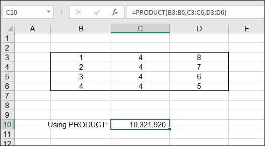
FIGURE 8-2: Putting the PRODUCT function to work.

Using What Remains with the MOD Function

The MOD function returns the remainder from an integer division operation. This remainder is called the modulus, hence the function’s name. The function has two arguments: the number being divided and the number being used to divide the first argument. The second argument is the divisor. The syntax follows:

=MOD(number, divisor)

These are examples of the MOD function:

• =MOD(12,6) returns 0.
• =MOD(14,5) returns 4.
• =MOD(27,7) returns 6.
• =MOD(25,10) returns 5.
• =MOD(25,-10) returns –5.
• =MOD(15.675,8.25) returns 7.425.

The returned value is always the same sign as the divisor.

You can use MOD to tell whether a number is odd or even. If you simply use a number 2 as the second argument, the returned value will be 0 if the first argument is an even number and 1 if it is not.

But what's so great about that? You can just look at a number and tell whether it’s odd or even. The power of the MOD function is apparent when you’re testing a reference or formula, such as =MOD(D12 - G15,2). In a complex worksheet with many formulas, you may not be able to tell when a cell will contain an odd or even number.

Taking this a step further, the MOD function can be used to identify cells in a worksheet that are multiples of the divisor. Figure 8-3 shows how this works.

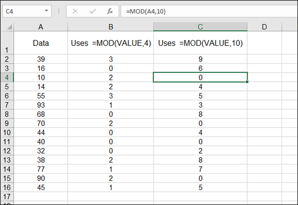
FIGURE 8-3: Using MOD to find specific values.

Row 1 of the worksheet in Figure 8-3 shows examples of the formulas that are entered in the successive rows of columns B and C, starting from the second row. Column A contains numbers that will be tested with the MOD function. If you’re looking for multiples of 4, the MOD function has 4 as the divisor, and when a value is a multiple of 4, MOD returns 0. This is evident when you compare the numbers in column A with the returned values in column B.

The same approach is used in column C, only here the divisor is 10, so multiples of 10 are being tested for in column A. Where a 0 appears in column C, the associated number in column A is a multiple of 10.

In this way, you can use the MOD function to find meaningful values in a worksheet.

Summing Things Up

Aha! Just when you think you know how to sum up numbers (really, haven’t you been doing this since your early school years?), I present a fancy-footwork summing that makes you think twice before going for that quick total.

The functions here are very cool — very “in” with the math crowd. To be a true Excel guru, try the SUBTOTAL, SUMPRODUCT, SUMIF, and SUMIFS functions shown here and then strut your stuff around the office!

Using SUBTOTAL

The SUBTOTAL function is very flexible. It doesn’t perform just one calculation; it can do any of 11 calculations depending on what you need. What’s more, SUBTOTAL can perform these calculations on up to 255 ranges of numbers. This gives you the ability to get exactly the type of summary you need without creating a complex set of formulas. The syntax of the function follows:

=SUBTOTAL(function number, range1, range2,…)

The first argument determines which calculation is performed. It can be any of the values shown in Table 8-3. The remaining arguments identify the ranges containing the numbers to be used in the calculation.

TABLE 8-3 Argument Values for the SUBTOTAL Function

Function Number for First Argument	Function	Description
1	AVERAGE	Returns the average value of a group of numbers
2	COUNT	Returns the count of cells that contain numbers and also numbers within the list of arguments
3	COUNTA	Returns the count of cells that are not empty and only nonempty values within the list of arguments
4	MAX	Returns the maximum value in a group of numbers
5	MIN	Returns the minimum value in a group of numbers
6	PRODUCT	Returns the product of a group of numbers
7	STDEV.S	Returns the standard deviation from a sample of values
8	STDEV.P	Returns the standard deviation from an entire population, including text and logical values
9	SUM	Returns the sum of a group of numbers
10	VAR.S	Returns variance based on a sample
11	VAR.P	Returns variance based on an entire population

Figure 8-4 show examples of using the SUBTOTAL function. Raw data values are listed in column A. The results of using the function in a few variations are listed in column C. Column E displays the actual function entries that returned the respective results in column C.

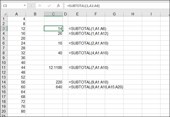
FIGURE 8-4: Working with the SUBTOTAL function.

Using named ranges with the SUBTOTAL function is useful. For example, =SUBTOTAL(1, October_Sales, November_Sales, December_sales) makes for an easy way to calculate the average sale of the fourth quarter.

A second set of numbers can be used for the Function Number (the first argument in the SUBTOTAL function). These numbers start with 101 and are the same functions as shown in Table 8-3. For example, 101 is AVERAGE, 102 is COUNT, and so on.

The 1 through 11 Function Numbers consider all values in a range. The 101 through 111 Function Numbers tell the function to ignore values that are in hidden rows or columns. Figure 8-5 shows SUBTOTAL in use with both Function Number systems. Comparing Figure 8-5 to Figure 8-4, you can see that row 2 has been set to hidden. In Figure 8-5, the values in column B are calculated using the same Function Numbers as in Figure 8-4; column G shows SUBTOTAL using the Function Numbers that start with 101. For example, cell B3 still shows the average of the numbers in the range A1:A6 as equal to 14. The result in cell G3 shows the average of A1:A6 equal to 15.2. The value of 8 in cell A2 is not used because it is hidden.

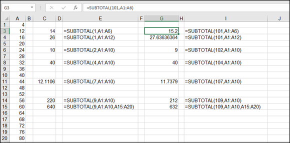
FIGURE 8-5: Getting SUBTOTAL to ignore hidden values.

Using SUMPRODUCT

The SUMPRODUCT function provides a sophisticated way to add various products — across ranges of values. It doesn't just add the products of separate ranges; it produces products of the values positioned in the same place in each range and then sums up those products. The syntax of the function follows:

=SUMPRODUCT(Range1, Range2, …)

The arguments to SUMPRODUCT must be ranges, although a range can be a single value. What is required is that all the ranges be the same size, both rows and columns. Up to 255 ranges are allowed, and at least 2 are required.

SUMPRODUCT works by first multiplying elements, by position, across the ranges and then adding all the results. To see how this works, take a look at the three ranges of values in Figure 8-6. I put letters in the ranges instead of numbers to make this easier to explain.

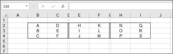
FIGURE 8-6: Following the steps used by SUMPRODUCT.

Suppose that you entered the following formula in the worksheet:

=SUMPRODUCT(B2:C4, E2:F4, H2:I4)

The result would be calculated by the following steps:

1. Multiplying A times H times N and saving the result
2. Multiplying D times K times Q and saving the result
3. Multiplying B times I times O and saving the result
4. Multiplying E times L times R and saving the result
5. Multiplying C times J times P and saving the result
6. Multiplying F times M times S and saving the result
7. Adding all six results to get the final answer

Be careful when you’re using the SUMPRODUCT function. It’s easy to mistakenly assume that the function adds products of individual ranges. It doesn’t. SUMPRODUCT returns the sums of products across positional elements.

As confusing as SUMPRODUCT seems, it actually has a sophisticated use. Imagine that you have a list of units sold by product and another list of the products’ prices. You need to know total sales (that is, the sum of the amounts), in which an amount is units sold times the unit price.

In the old days of spreadsheets, you would use an additional column to first multiply each unit sold figure by its price. Then you would sum those intermediate values. Now, with SUMPRODUCT, the drudgery is over. The single use of SUMPRODUCT gets the final answer in one step. Figure 8-7 shows how one cell contains the needed grand total. No intermediate steps are necessary.

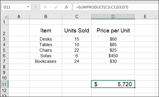
FIGURE 8-7: Being productive with SUMPRODUCT.

Using SUMIF and SUMIFS

SUMIF is one of the real gemstones of Excel functions. It calculates the sum of a range of values, including only those values that meet a specified criterion. The criterion can be based on the same column that is being summed, or it can be based on an adjacent column.

Suppose that you use a worksheet to keep track of all your food-store purchases. For each shopping trip, you put the date in column A, the amount in column B, and the name of the store in column C. You can use the SUMIF function to tell Excel to add all the values in column B only where column C contains "Great Grocery". That’s it. SUMIF gives you the answer. Neat!

Figure 8-8 shows this example. The date of purchase, place of purchase, and amount spent are listed in three columns. SUMIF calculates the sum of purchases at Great Grocery. Here is how the function is written for the example:

=SUMIF(C3:C15,"Great Grocery",B3:B15)

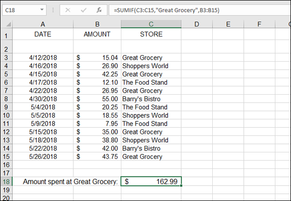
FIGURE 8-8: Using SUMIF for targeted tallying.

Here are a couple of important points about the SUMIF function:

• The second argument can accommodate several variations of expressions, such as including greater than (>) or less than (<) signs or other operators. For example, if a column has regions such as North, South, East, and West, the criteria could be <>North, which would return the sum of rows that are not for the North region.
• Unpredictable results occur if the ranges in the first and third arguments do not match in size.

Try it yourself! Here’s how to use the SUMIF function:

1. Enter two ranges of data in a worksheet.

   At least one should contain numerical data. Make sure both ranges are the same size.

2. Position the pointer in the cell where you want the results displayed.
3. Type =SUMIF( to begin the function.

4. Hold down the left mouse button and drag the pointer over one of the ranges.

   This is the range that can be other than numerical data.

5. Type a comma (,).

6. Click one of the cells in the first range.

   This is the criterion.

7. Type a comma (,).

8. Hold down the left mouse button and drag the pointer over the second range.

   This is the range that must contain numerical data.

9. Type a ) and press Enter.

The result you see is a sum of the numeric values where the items in the first range matched the selected criteria.

The example in Figure 8-8 sums values when the store is Great Grocery but does not use the date in the calculation. What if you need to know how much was spent at Great Grocery in April only? Excel provides a function for this, of course: SUMIFS.

SUMIFS lets you apply multiple “if” conditions to a sum. The format of SUMIFS is a bit different from SUMIF. SUMIFS uses this structure:

=SUMIFS(range to be summed, criteria range 1, criteria 1, criteria range 2, criteria 2)

The structure requires the range of numerical values to be entered first, followed by pairs of criteria ranges and the criteria itself. In Figure 8-9, the formula is

=SUMIFS(B3:B15,A3:A15,"<5/1/2018",C3:C15,"Great Grocery")

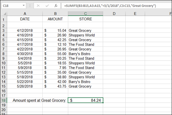
FIGURE 8-9: Using SUMIFS to get a multiple filtered sum.

The function uses B3:B15 as the source of values to sum. A1:A15 is the first criteria range, and “<5/1/2018” is the criteria. This tells the function to look for any date that is earlier than May 1, 2018 (which filters the dates to just April). This is followed by a second criteria range and value: In C3:C15, look just for Great Grocery. The final sum of $84.24 adds just three numbers — 15.04, 42.25, and 26.95 — because these are the only values in April for Great Grocery.

Getting an Angle on Trigonometry

Did you think Excel was not up to snuff to provide some tricks for trigonometry? Then think again. Who can resist playing around with such exciting things like cosines and tangents? All right, I admit this is not for everyone, but here are the trig functions nonetheless. Besides, even if the concepts are difficult, you can always throw around the terms at a party and be recognized as the brainiest person there.

Three basic trigonometry functions

The sine, cosine, and tangent of an angle are likely the most used values in trigonometry calculations. They provide answers about the relationships of a triangle’s angles to the sides of the triangle. (See how I boiled down the bulk of trigonometry into a single sentence!)

Figure 8-10 shows a handful of angles in column A and their corresponding sine, cosine, and tangent values in columns B, C, and D, respectively.

FIGURE 8-10: Using SIN, COS, and TAN functions.

The SIN, COS, and TAN functions take just the single argument of a number (the angle) and return the converted values. The functions look like this if the angles are in radians:

=SIN(angle)
=COS(angle)
=TAN(angle)

If the angles are in degrees, they need to be converted to radians by the RADIANS function. In this case, you would use these:

=SIN(RADIANS(angle))
=COS(RADIANS(angle))
=TAN(RADIANS(angle))

Which leads you to …

Degrees and radians

An angle can be expressed in degrees or radians. A degree is more common to us non–rocket scientists. Most everyone know that there are 360 degrees in a circle, that a right angle is 90 degrees, and even that “doing a 180” means turning completely around and going the other way.

One radian = 180/pi degrees, and one degree = pi/180 radians. All this talk about pi is making me hungry! For lowdown and quick conversion: 1 radian = 57.3 degrees.

Pi is approximately equal to 3.14159. See the beginning of this chapter for a forkful of pi.

Excel provides the RADIANS and DEGREES functions to convert a number from radians to degrees or vice versa. I think the real reason Excel did this was to keep pi out of the picture so you would concentrate on work and not dessert.

The functions are the single argument type:

=RADIANS(angle in degrees)
=DEGREES(angle in radians)

Using some numbers, you can see that 90 degrees = 1.5707963267949 radians and so 1.5707963267949 radians must equal 90 degrees. And it does.